pseudo-spectral representations

(0.002 seconds)

11—20 of 177 matching pages

11: 13.27 Mathematical Applications

… ►Confluent hypergeometric functions are connected with representations of the group of third-order triangular matrices. …Vilenkin (1968, Chapter 8) constructs irreducible representations of this group, in which the diagonal matrices correspond to operators of multiplication by an exponential function. …

12: 14.32 Methods of Computation

… ►In particular, for small or moderate values of the parameters

\mu

and

\nu

the power-series expansions of the various hypergeometric function representations given in §§14.3(i)–14.3(iii), 14.19(ii), and 14.20(i) can be selected in such a way that convergence is stable, and reasonably rapid, especially when the argument of the functions is real. … ►

•

Quadrature (§3.5) of the integral representations given in §§14.12, 14.19(iii), 14.20(iv), and 14.25; see Segura and Gil (1999) and Gil et al. (2000).

…

13: 34.6 Definition: $\mathit{9j}$ Symbol

… ►The

\mathit{9j}

symbol may be defined either in terms of

\mathit{3j}

symbols or equivalently in terms of

\mathit{6j}

symbols: ►

34.6.1

\begin{Bmatrix}j_{11}&j_{12}&j_{13}\\ j_{21}&j_{22}&j_{23}\\ j_{31}&j_{32}&j_{33}\end{Bmatrix}=\sum_{\mbox{\scriptsize all }m_{rs}}\begin{% pmatrix}j_{11}&j_{12}&j_{13}\\ m_{11}&m_{12}&m_{13}\end{pmatrix}\begin{pmatrix}j_{21}&j_{22}&j_{23}\\ m_{21}&m_{22}&m_{23}\end{pmatrix}\begin{pmatrix}j_{31}&j_{32}&j_{33}\\ m_{31}&m_{32}&m_{33}\end{pmatrix}\*\begin{pmatrix}j_{11}&j_{21}&j_{31}\\ m_{11}&m_{21}&m_{31}\end{pmatrix}\begin{pmatrix}j_{12}&j_{22}&j_{32}\\ m_{12}&m_{22}&m_{32}\end{pmatrix}\begin{pmatrix}j_{13}&j_{23}&j_{33}\\ m_{13}&m_{23}&m_{33}\end{pmatrix},

ⓘ

Defines:: $\begin{Bmatrix}\NVar{j_{11}}&\NVar{j_{12}}&\NVar{j_{13}}\\ \NVar{j_{21}}&\NVar{j_{22}}&\NVar{j_{23}}\\ \NVar{j_{31}}&\NVar{j_{32}}&\NVar{j_{33}}\end{Bmatrix}$ : $\mathit{9j}$ symbol
Symbols:: $\begin{pmatrix}\NVar{j_{1}}&\NVar{j_{2}}&\NVar{j_{3}}\\ \NVar{m_{1}}&\NVar{m_{2}}&\NVar{m_{3}}\end{pmatrix}$ : $\mathit{3j}$ symbol, $j,j_{r}$ : non-negative integers or non-negative integers plus one half., $r$ : nonnegative integer and $s$ : integer
Permalink:: http://dlmf.nist.gov/34.6.E1
Encodings:: pMML, png, TeX
See also:: Annotations for §34.6 and Ch.34

… ►The

\mathit{9j}

symbol may also be written as a finite triple sum equivalent to a terminating generalized hypergeometric series of three variables with unit arguments. …

14: 1.17 Integral and Series Representations of the Dirac Delta

§1.17 Integral and Series Representations of the Dirac Delta

… ►

§1.17(ii) Integral Representations

… ►Then comparison of (1.17.2) and (1.17.9) yields the formal integral representation … ►

Sine and Cosine Functions

… ►

§1.17(iii) Series Representations

…

15: 14.25 Integral Representations

§14.25 Integral Representations

… ►For corresponding contour integrals, with less restrictions on

\mu

and

\nu

, see Olver (1997b, pp. 174–179), and for further integral representations see Magnus et al. (1966, §4.6.1).

16: 24.7 Integral Representations

§24.7 Integral Representations

►

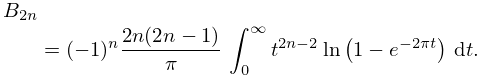
§24.7(i) Bernoulli and Euler Numbers

… ►

24.7.5

B_{2n}=(-1)^{n}\frac{2n(2n-1)}{\pi}\*\int_{0}^{\infty}t^{2n-2}\ln\left(1-e^{-2% \pi t}\right)\,\mathrm{d}t.

ⓘ

Symbols:: $B_{\NVar{n}}$ : Bernoulli numbers, $\pi$ : the ratio of the circumference of a circle to its diameter, $\,\mathrm{d}\NVar{x}$ : differential of $x$ , $\mathrm{e}$ : base of natural logarithm, $\int$ : integral, $\ln\NVar{z}$ : principal branch of logarithm function, $n$ : integer and $t$ : real or complex
Referenced by:: §24.7(i)
Permalink:: http://dlmf.nist.gov/24.7.E5
Encodings:: pMML, png, TeX
See also:: Annotations for §24.7(i), §24.7 and Ch.24

… ►

§24.7(ii) Bernoulli and Euler Polynomials

… ►For further integral representations see Prudnikov et al. (1986a, §§2.3–2.6) and Gradshteyn and Ryzhik (2000, Chapters 3 and 4).

17: 25.5 Integral Representations

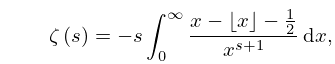
§25.5 Integral Representations

… ►

25.5.5

\zeta\left(s\right)=-s\int_{0}^{\infty}\frac{x-\left\lfloor x\right\rfloor-% \frac{1}{2}}{x^{s+1}}\,\mathrm{d}x,

-1<\Re s<0

ⓘ

Symbols:: $\zeta\left(\NVar{s}\right)$ : Riemann zeta function, $\,\mathrm{d}\NVar{x}$ : differential of $x$ , $\left\lfloor\NVar{x}\right\rfloor$ : floor of $x$ , $\int$ : integral, $\Re$ : real part, $x$ : real variable and $s$ : complex variable
Keywords:: improper integral, integral representation
Source:: Titchmarsh (1986b, (2.1.6), p. 15)
Permalink:: http://dlmf.nist.gov/25.5.E5
Encodings:: pMML, png, TeX
See also:: Annotations for §25.5(i), §25.5 and Ch.25

… ►For similar representations involving other theta functions see Erdélyi et al. (1954a, p. 339). … ►

25.5.19

\zeta\left(m+s\right)=(-1)^{m-1}\frac{\Gamma\left(s\right)\sin\left(\pi s% \right)}{\pi\Gamma\left(m+s\right)}\*\int_{0}^{\infty}{\psi}^{(m)}\left(1+x% \right)x^{-s}\,\mathrm{d}x,

m=1,2,3,\dots

ⓘ

Symbols:: $\Gamma\left(\NVar{z}\right)$ : gamma function, $\zeta\left(\NVar{s}\right)$ : Riemann zeta function, $\pi$ : the ratio of the circumference of a circle to its diameter, $\,\mathrm{d}\NVar{x}$ : differential of $x$ , $\psi\left(\NVar{z}\right)$ : psi (or digamma) function, $\int$ : integral, $\sin\NVar{z}$ : sine function, $m$ : nonnegative integer, $x$ : real variable and $s$ : complex variable
Keywords:: improper integral, integral representation
Source:: de Bruijn (1937, p. 178)
Referenced by:: §25.5(ii)
Permalink:: http://dlmf.nist.gov/25.5.E19
Encodings:: pMML, png, TeX
See also:: Annotations for §25.5(ii), §25.5 and Ch.25

►

§25.5(iii) Contour Integrals

…

18: 14.26 Uniform Asymptotic Expansions

… ►See also Frenzen (1990), Gil et al. (2000), Shivakumar and Wong (1988), Ursell (1984), and Wong (1989) for uniform asymptotic approximations obtained from integral representations.

19: 23.11 Integral Representations

§23.11 Integral Representations

…

20: 35.10 Methods of Computation

… ►Other methods include numerical quadrature applied to double and multiple integral representations. …