partial pivoting

SearchAdvancedHelp

(0.002 seconds)

1—10 of 95 matching pages

1: 3.2 Linear Algebra

… ►To avoid instability the rows are interchanged at each elimination step in such a way that the absolute value of the element that is used as a divisor, the pivot element, is not less than that of the other available elements in its column. …This modification is called Gaussian elimination with partial pivoting. ►For more information on pivoting see Golub and Van Loan (1996, pp. 109–123). … ►Assume that $𝐀$ can be factored as in (3.2.5), but without partial pivoting. …

2: 36.10 Differential Equations

… ►

§36.10(ii) Partial Derivatives with Respect to the $x_n$

… ►

36.10.7 $$\frac{{\partial }^{2n}{\mathrm{\Psi }}_2}{{\partial x}^{2n}}={\mathrm{i}}^n\frac{{\partial }^n{\mathrm{\Psi }}_2}{{\partial y}^n}.$$

ⓘ

Symbols:

${\mathrm{\Psi }}_K\left(𝐱\right)$: canonical integral function, $\mathrm{i}$: imaginary unit, $\frac{\partial f}{\partial x}$: partial derivative of $f$ with respect to $x$ , $\partial x$: partial differential of $x$ , $y$: real parameter, $m$: integer and $x$: real parameter

Permalink:

http://dlmf.nist.gov/36.10.E7

Encodings:

pMML, png, TeX

See also:

Annotations for §36.10(ii), §36.10(ii), §36.10 and Ch.36

… ►

36.10.8 $$\frac{{\partial }^{2n}{\mathrm{\Psi }}_3}{{\partial x}^{2n}}={\mathrm{i}}^n\frac{{\partial }^n{\mathrm{\Psi }}_3}{{\partial y}^n},$$

ⓘ

Symbols:

${\mathrm{\Psi }}_K\left(𝐱\right)$: canonical integral function, $\mathrm{i}$: imaginary unit, $\frac{\partial f}{\partial x}$: partial derivative of $f$ with respect to $x$ , $\partial x$: partial differential of $x$ , $y$: real parameter, $m$: integer and $x$: real parameter

Permalink:

http://dlmf.nist.gov/36.10.E8

Encodings:

pMML, png, TeX

See also:

Annotations for §36.10(ii), §36.10(ii), §36.10 and Ch.36

… ►

36.10.10 $$\frac{{\partial }^{3n}{\mathrm{\Psi }}_3}{{\partial y}^{3n}}={\mathrm{i}}^n\frac{{\partial }^{2n}{\mathrm{\Psi }}_3}{{\partial z}^{2n}}.$$

ⓘ

Symbols:

${\mathrm{\Psi }}_K\left(𝐱\right)$: canonical integral function, $\mathrm{i}$: imaginary unit, $\frac{\partial f}{\partial x}$: partial derivative of $f$ with respect to $x$ , $\partial x$: partial differential of $x$ , $y$: real parameter, $z$: real parameter and $m$: integer

Permalink:

http://dlmf.nist.gov/36.10.E10

Encodings:

pMML, png, TeX

See also:

Annotations for §36.10(ii), §36.10(ii), §36.10 and Ch.36

… ►

§36.10(iv) Partial $z$-Derivatives

…

3: 1.5 Calculus of Two or More Variables

… ►

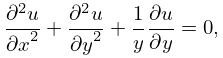
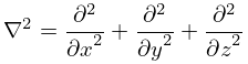
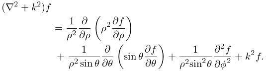
§1.5(i) Partial Derivatives

… ►The function $f(x,y)$ is continuously differentiable if $f$, $\partial f/\partial x$, and $\partial f/\partial y$ are continuous, and twice-continuously differentiable if also ${\partial }^{2}f/{\partial x}^2$, ${\partial }^{2}f/{\partial y}^2$, ${\partial }^{2}f/\partial x\partial y$, and ${\partial }^{2}f/\partial y\partial x$ are continuous. … ►Sufficient conditions for validity are: (a) $f$ and $\partial f/\partial x$ are continuous on a rectangle $a\le x\le b$, $c\le y\le d$; (b) when $x\in [a,b]$ both $\alpha (x)$ and $\beta (x)$ are continuously differentiable and lie in $[c,d]$. … ►Suppose that $a,b,c$ are finite, $d$ is finite or $+\mathrm{\infty }$, and $f(x,y)$, $\partial f/\partial x$ are continuous on the partly-closed rectangle or infinite strip $[a,b]\times [c,d)$. Suppose also that ${\int }_c^{d}f(x,y)dy$ converges and ${\int }_c^d(\partial f/\partial x)dy$ converges uniformly on $a\le x\le b$, that is, given any positive number $ϵ$, however small, we can find a number $c_0\in [c,d)$ that is independent of $x$ and is such that …

4: 19.18 Derivatives and Differential Equations

… ►Let ${\partial }_j=\partial /\partial z_j$, and ${𝐞}_j$ be an $n$-tuple with 1 in the $j$th place and 0’s elsewhere. … ►If $n=2$, then elimination of ${\partial }_{2}v$ between (19.18.11) and (19.18.12), followed by the substitution $(b_1,b_2,z_1,z_2)=(b,c-b,1-z,1)$, produces the Gauss hypergeometric equation (15.10.1). … ►

19.18.14 $$\frac{{\partial }^{2}w}{{\partial x}^2}=\frac{{\partial }^{2}w}{{\partial y}^2}+\frac{1}{y}\frac{\partial w}{\partial y}.$$

ⓘ

Symbols:

$\frac{\partial f}{\partial x}$: partial derivative of $f$ with respect to $x$ and $\partial x$: partial differential of $x$

Permalink:

http://dlmf.nist.gov/19.18.E14

Encodings:

pMML, png, TeX

See also:

Annotations for §19.18(ii), §19.18 and Ch.19

… ►

19.18.15 $$\frac{{\partial }^{2}W}{{\partial t}^2}=\frac{{\partial }^{2}W}{{\partial x}^2}+\frac{{\partial }^{2}W}{{\partial y}^2}.$$

ⓘ

Symbols:

$\frac{\partial f}{\partial x}$: partial derivative of $f$ with respect to $x$ , $\partial x$: partial differential of $x$ and $W$: wave function

Permalink:

http://dlmf.nist.gov/19.18.E15

Encodings:

pMML, png, TeX

See also:

Annotations for §19.18(ii), §19.18 and Ch.19

… ►

19.18.16 $$\frac{{\partial }^{2}u}{{\partial x}^2}+\frac{{\partial }^{2}u}{{\partial y}^2}+\frac{1}{y}\frac{\partial u}{\partial y}=0,$$

ⓘ

Symbols:

$\frac{\partial f}{\partial x}$: partial derivative of $f$ with respect to $x$ and $\partial x$: partial differential of $x$

Permalink:

http://dlmf.nist.gov/19.18.E16

Encodings:

pMML, png, TeX

See also:

Annotations for §19.18(ii), §19.18 and Ch.19

…

5: 16.14 Partial Differential Equations

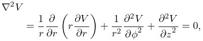
§16.14 Partial Differential Equations

►

§16.14(i) Appell Functions

►

$$x(1-x)\frac{{\partial }^2{F}_1}{{\partial x}^2}+y(1-x)\frac{{\partial }^2{F}_1}{\partial x\partial y}+\left(\gamma -(\alpha +\beta +1)x\right)\frac{\partial F_1}{\partial x}-\beta y\frac{\partial F_1}{\partial y}-\alpha \beta F_1=0,$$

►

$$y(1-y)\frac{{\partial }^2{F}_1}{{\partial y}^2}+x(1-y)\frac{{\partial }^2{F}_1}{\partial x\partial y}+\left(\gamma -(\alpha +{\beta }^{\prime }+1)y\right)\frac{\partial F_1}{\partial y}-{\beta }^{\prime }x\frac{\partial F_1}{\partial x}-\alpha {\beta }^{\prime }{F}_1=0,$$

… ►In addition to the four Appell functions there are $24$ other sums of double series that cannot be expressed as a product of two ${}_2{}^{}F_1^{}$ functions, and which satisfy pairs of linear partial differential equations of the second order. …

6: 10.38 Derivatives with Respect to Order

… ►

10.38.2 $$\frac{\partial K_{\nu }\left(z\right)}{\partial \nu }=\frac{1}{2}\pi \csc \left(\nu \pi \right)\left(\frac{\partial I_{-\nu }\left(z\right)}{\partial \nu }-\frac{\partial I_{\nu }\left(z\right)}{\partial \nu }\right)-\pi \cot \left(\nu \pi \right)K_{\nu }\left(z\right),$$ $\nu \notin \mathbb{Z}$.

ⓘ

Symbols:

$\pi$: the ratio of the circumference of a circle to its diameter, $\csc z$: cosecant function, $\cot z$: cotangent function, $\mathbb{Z}$: set of all integers, $I_{\nu }\left(z\right)$: modified Bessel function of the first kind, $K_{\nu }\left(z\right)$: modified Bessel function of the second kind, $\notin$: not an element of, $\frac{\partial f}{\partial x}$: partial derivative of $f$ with respect to $x$ , $\partial x$: partial differential of $x$ , $z$: complex variable and $\nu$: complex parameter

A&S Ref:

9.6.43

Referenced by:

(10.38.1), §10.38, §10.38

Permalink:

http://dlmf.nist.gov/10.38.E2

Encodings:

pMML, png, TeX

See also:

Annotations for §10.38 and Ch.10

… ►For $\partial I_{\nu }\left(z\right)/\partial \nu$ at $\nu =-n$ combine (10.38.1), (10.38.2), and (10.38.4). ►

10.38.4 $${\frac{\partial K_{\nu }\left(z\right)}{\partial \nu }|}_{\nu =n}=\frac{n!}{2{(\frac{1}{2}z)}^n}\sum _{k=0}^{n-1}\frac{{(\frac{1}{2}z)}^k{K}_k\left(z\right)}{k!(n-k)}.$$

ⓘ

Symbols:

$!$: factorial (as in $n!$), $K_{\nu }\left(z\right)$: modified Bessel function of the second kind, $\frac{\partial f}{\partial x}$: partial derivative of $f$ with respect to $x$ , $\partial x$: partial differential of $x$ , $n$: integer, $k$: nonnegative integer, $z$: complex variable and $\nu$: complex parameter

A&S Ref:

9.6.45

Referenced by:

§10.38

Permalink:

http://dlmf.nist.gov/10.38.E4

Encodings:

pMML, png, TeX

See also:

Annotations for §10.38, §10.38 and Ch.10

►

${{\displaystyle \frac{\partial I_{\nu }\left(z\right)}{\partial \nu }}|}_{\nu =0}=-K_0\left(z\right),$

… ►

10.38.7 $${\frac{\partial K_{\nu }\left(x\right)}{\partial \nu }|}_{\nu =\pm \frac{1}{2}}=\pm \sqrt{\frac{\pi }{2x}}{E}_1\left(2x\right){\mathrm{e}}^x.$$

ⓘ

Symbols:

$\pi$: the ratio of the circumference of a circle to its diameter, $\mathrm{e}$: base of natural logarithm, $E_1\left(z\right)$: exponential integral, $K_{\nu }\left(z\right)$: modified Bessel function of the second kind, $\frac{\partial f}{\partial x}$: partial derivative of $f$ with respect to $x$ , $\partial x$: partial differential of $x$ , $x$: real variable and $\nu$: complex parameter

A&S Ref:

10.2.34 (corrected)

Referenced by:

§10.38, Ch.10

Permalink:

http://dlmf.nist.gov/10.38.E7

Encodings:

pMML, png, TeX

See also:

Annotations for §10.38, §10.38 and Ch.10

…

7: 10.15 Derivatives with Respect to Order

… ►

10.15.1 $$\frac{\partial J_{\pm \nu }\left(z\right)}{\partial \nu }=\pm J_{\pm \nu }\left(z\right)\ln \left(\frac{1}{2}z\right)\mp {(\frac{1}{2}z)}^{\pm \nu }\sum _{k=0}^{\mathrm{\infty }}{(-1)}^k\frac{\psi \left(k+1\pm \nu \right)}{\mathrm{\Gamma }\left(k+1\pm \nu \right)}\frac{{(\frac{1}{4}{z}^2)}^k}{k!},$$

ⓘ

Symbols:

$J_{\nu }\left(z\right)$: Bessel function of the first kind, $\mathrm{\Gamma }\left(z\right)$: gamma function, $\psi \left(z\right)$: psi (or digamma) function, $!$: factorial (as in $n!$), $\ln z$: principal branch of logarithm function, $\frac{\partial f}{\partial x}$: partial derivative of $f$ with respect to $x$ , $\partial x$: partial differential of $x$ , $k$: nonnegative integer, $z$: complex variable and $\nu$: complex parameter

A&S Ref:

9.1.64

Referenced by:

§10.15, §10.38, Erratum (V1.0.17) for Equations (10.15.1), (10.38.1)

Permalink:

http://dlmf.nist.gov/10.15.E1

Encodings:

pMML, png, TeX

Addition (effective with 1.0.17):

This equation has been generalized to include the additional case of $\partial J_{-\nu }\left(z\right)/\partial \nu$ because it will help the user who wants to combine it with (10.15.2).

See also:

Annotations for §10.15, §10.15 and Ch.10

►

10.15.2 $$\frac{\partial Y_{\nu }\left(z\right)}{\partial \nu }=\cot \left(\nu \pi \right)\left(\frac{\partial J_{\nu }\left(z\right)}{\partial \nu }-\pi Y_{\nu }\left(z\right)\right)-\csc \left(\nu \pi \right)\frac{\partial J_{-\nu }\left(z\right)}{\partial \nu }-\pi J_{\nu }\left(z\right).$$

ⓘ

Symbols:

$J_{\nu }\left(z\right)$: Bessel function of the first kind, $Y_{\nu }\left(z\right)$: Bessel function of the second kind, $\pi$: the ratio of the circumference of a circle to its diameter, $\csc z$: cosecant function, $\cot z$: cotangent function, $\frac{\partial f}{\partial x}$: partial derivative of $f$ with respect to $x$ , $\partial x$: partial differential of $x$ , $z$: complex variable and $\nu$: complex parameter

A&S Ref:

9.1.65

Referenced by:

(10.15.1), §10.15

Permalink:

http://dlmf.nist.gov/10.15.E2

Encodings:

pMML, png, TeX

See also:

Annotations for §10.15, §10.15 and Ch.10

… ►

10.15.3 $${\frac{\partial J_{\nu }\left(z\right)}{\partial \nu }|}_{\nu =n}=\frac{\pi }{2}{Y}_n\left(z\right)+\frac{n!}{2{(\frac{1}{2}z)}^n}\sum _{k=0}^{n-1}\frac{{(\frac{1}{2}z)}^k{J}_k\left(z\right)}{k!(n-k)}.$$

ⓘ

Symbols:

$J_{\nu }\left(z\right)$: Bessel function of the first kind, $Y_{\nu }\left(z\right)$: Bessel function of the second kind, $\pi$: the ratio of the circumference of a circle to its diameter, $!$: factorial (as in $n!$), $\frac{\partial f}{\partial x}$: partial derivative of $f$ with respect to $x$ , $\partial x$: partial differential of $x$ , $n$: integer, $k$: nonnegative integer, $z$: complex variable and $\nu$: complex parameter

A&S Ref:

9.1.66

Referenced by:

§10.15, §10.15, §10.38

Permalink:

http://dlmf.nist.gov/10.15.E3

Encodings:

pMML, png, TeX

See also:

Annotations for §10.15, §10.15 and Ch.10

►For $\partial J_{\nu }\left(z\right)/\partial \nu$ at $\nu =-n$ combine (10.2.4) and (10.15.3). … ►

10.15.5 $${\frac{\partial J_{\nu }\left(z\right)}{\partial \nu }|}_{\nu =0}=\frac{\pi }{2}{Y}_0\left(z\right),{\frac{\partial Y_{\nu }\left(z\right)}{\partial \nu }|}_{\nu =0}=-\frac{\pi }{2}{J}_0\left(z\right).$$

ⓘ

Symbols:

$J_{\nu }\left(z\right)$: Bessel function of the first kind, $Y_{\nu }\left(z\right)$: Bessel function of the second kind, $\pi$: the ratio of the circumference of a circle to its diameter, $\frac{\partial f}{\partial x}$: partial derivative of $f$ with respect to $x$ , $\partial x$: partial differential of $x$ , $z$: complex variable and $\nu$: complex parameter

A&S Ref:

9.1.68

Referenced by:

§10.15, §10.38

Permalink:

http://dlmf.nist.gov/10.15.E5

Encodings:

pMML, png, TeX

See also:

Annotations for §10.15, §10.15 and Ch.10

…

8: 12.17 Physical Applications

… ►

12.17.2 $${\nabla }^2=\frac{{\partial }^2}{{\partial x}^2}+\frac{{\partial }^2}{{\partial y}^2}+\frac{{\partial }^2}{{\partial z}^2}$$

ⓘ

Symbols:

$\frac{\partial f}{\partial x}$: partial derivative of $f$ with respect to $x$ , $\partial x$: partial differential of $x$ , $x$: real variable, $y$: real variable and $z$: complex variable

Permalink:

http://dlmf.nist.gov/12.17.E2

Encodings:

pMML, png, TeX

See also:

Annotations for §12.17 and Ch.12

… ►

12.17.4 $$\frac{1}{{\xi }^2+{\eta }^2}\left(\frac{{\partial }^{2}w}{{\partial \xi }^2}+\frac{{\partial }^{2}w}{{\partial \eta }^2}\right)+\frac{{\partial }^{2}w}{{\partial \zeta }^2}+k^{2}w=0.$$

ⓘ

Symbols:

$\frac{\partial f}{\partial x}$: partial derivative of $f$ with respect to $x$ , $\partial x$: partial differential of $x$ , $k$: constant, $\xi$: coordinate, $\eta$: coordinate and $\zeta$: coordinate

Permalink:

http://dlmf.nist.gov/12.17.E4

Encodings:

pMML, png, TeX

See also:

Annotations for §12.17 and Ch.12

…

9: 10.73 Physical Applications

… ►

10.73.1 $${\nabla }^{2}V=\frac{1}{r}\frac{\partial }{\partial r}\left(r\frac{\partial V}{\partial r}\right)+\frac{1}{r^2}\frac{{\partial }^{2}V}{{\partial \varphi }^2}+\frac{{\partial }^{2}V}{{\partial z}^2}=0,$$

ⓘ

Symbols:

$\frac{\partial f}{\partial x}$: partial derivative of $f$ with respect to $x$ and $\partial x$: partial differential of $x$

Permalink:

http://dlmf.nist.gov/10.73.E1

Encodings:

pMML, png, TeX

See also:

Annotations for §10.73(i), §10.73 and Ch.10

… ►

10.73.2 $${\nabla }^2\psi =\frac{1}{c^2}\frac{{\partial }^2\psi }{{\partial t}^2},$$

ⓘ

Symbols:

$\frac{\partial f}{\partial x}$: partial derivative of $f$ with respect to $x$ and $\partial x$: partial differential of $x$

Permalink:

http://dlmf.nist.gov/10.73.E2

Encodings:

pMML, png, TeX

See also:

Annotations for §10.73(i), §10.73 and Ch.10

… ►

10.73.3 $${\nabla }^{4}W+{\lambda }^2\frac{{\partial }^{2}W}{{\partial t}^2}=0.$$

ⓘ

Symbols:

$\frac{\partial f}{\partial x}$: partial derivative of $f$ with respect to $x$ and $\partial x$: partial differential of $x$

Permalink:

http://dlmf.nist.gov/10.73.E3

Encodings:

pMML, png, TeX

See also:

Annotations for §10.73(i), §10.73 and Ch.10

… ►

10.73.4 $$({\nabla }^2+k^2)f=\frac{1}{{\rho }^2}\frac{\partial }{\partial \rho }\left({\rho }^2\frac{\partial f}{\partial \rho }\right)+\frac{1}{{\rho }^2\sin \theta }\frac{\partial }{\partial \theta }\left(\sin \theta \frac{\partial f}{\partial \theta }\right)+\frac{1}{{\rho }^2{\sin }^2\theta }\frac{{\partial }^{2}f}{{\partial \varphi }^2}+k^{2}f.$$

ⓘ

Symbols:

$\frac{\partial f}{\partial x}$: partial derivative of $f$ with respect to $x$ , $\partial x$: partial differential of $x$ , $\sin z$: sine function and $k$: nonnegative integer

Permalink:

http://dlmf.nist.gov/10.73.E4

Encodings:

pMML, png, TeX

See also:

Annotations for §10.73(ii), §10.73 and Ch.10

…

10: 23.21 Physical Applications

… ►

§23.21(ii) Nonlinear Evolution Equations

►Airault et al. (1977) applies the function $\mathrm{\wp }$ to an integrable classical many-body problem, and relates the solutions to nonlinear partial differential equations. … ►

23.21.2 $$(\eta -\zeta )(\zeta -\xi )(\xi -\eta ){\nabla }^2=(\zeta -\eta )f(\xi )f^{\prime }(\xi )\frac{\partial }{\partial \xi }+(\xi -\zeta )f(\eta )f^{\prime }(\eta )\frac{\partial }{\partial \eta }+(\eta -\xi )f(\zeta )f^{\prime }(\zeta )\frac{\partial }{\partial \zeta },$$

ⓘ

Symbols:

$\frac{\partial f}{\partial x}$: partial derivative of $f$ with respect to $x$ , $\partial x$: partial differential of $x$ , $\xi$: ellipsoidal coordinate, $\eta$: ellipsoidal coordinate, $\zeta$: ellipsoidal coordinate and $f(\rho )$: function

Permalink:

http://dlmf.nist.gov/23.21.E2

Encodings:

pMML, png, TeX

See also:

Annotations for §23.21(iii), §23.21 and Ch.23

… ►

23.21.5 $$\left(\mathrm{\wp }\left(v\right)-\mathrm{\wp }\left(w\right)\right)\left(\mathrm{\wp }\left(w\right)-\mathrm{\wp }\left(u\right)\right)\left(\mathrm{\wp }\left(u\right)-\mathrm{\wp }\left(v\right)\right){\nabla }^2=\left(\mathrm{\wp }\left(w\right)-\mathrm{\wp }\left(v\right)\right)\frac{{\partial }^2}{{\partial u}^2}+\left(\mathrm{\wp }\left(u\right)-\mathrm{\wp }\left(w\right)\right)\frac{{\partial }^2}{{\partial v}^2}+\left(\mathrm{\wp }\left(v\right)-\mathrm{\wp }\left(u\right)\right)\frac{{\partial }^2}{{\partial w}^2}.$$

ⓘ

Symbols:

$\mathrm{\wp }\left(z\right)$ (= $\mathrm{\wp }\left(z|𝕃\right)$ = $\mathrm{\wp }(z;g_2,g_3)$): Weierstrass $\mathrm{\wp }$-function, $\frac{\partial f}{\partial x}$: partial derivative of $f$ with respect to $x$ , $\partial x$: partial differential of $x$ , $𝕃$: lattice, $u$: change of variable, $v$: change of variable and $w$: change of variable

Permalink:

http://dlmf.nist.gov/23.21.E5

Encodings:

pMML, png, TeX

See also:

Annotations for §23.21(iii), §23.21 and Ch.23

…