big q-Jacobi polynomials
(0.001 seconds)
21—30 of 314 matching pages
21: 8.27 Approximations
…
►
•
…
►
•
…
►
•
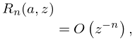
DiDonato (1978) gives a simple approximation for the function (which is related to the incomplete gamma function by a change of variables) for real and large positive . This takes the form , approximately, where and is shown to produce an absolute error as .
Luke (1969b, p. 186) gives hypergeometric polynomial representations that converge uniformly on compact subsets of the -plane that exclude and are valid for .
Verbeeck (1970) gives polynomial and rational approximations for , approximately, where denotes a quotient of polynomials of equal degree in .
22: 2.8 Differential Equations with a Parameter
…
►For example, can be the order of a Bessel function or degree of an orthogonal polynomial.
…
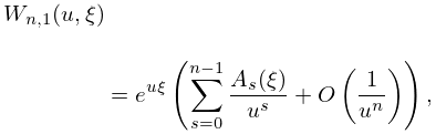
►
2.8.11
,
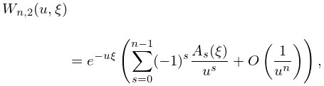
►
2.8.12
,
…
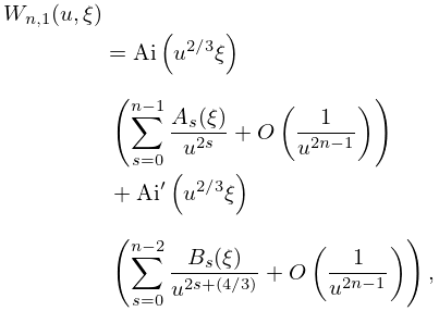
►
2.8.15
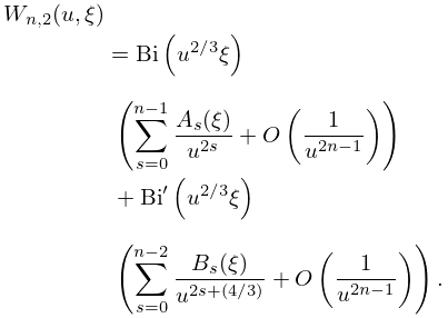
►
2.8.16
…
23: 19.27 Asymptotic Approximations and Expansions
24: 27.11 Asymptotic Formulas: Partial Sums
…
►
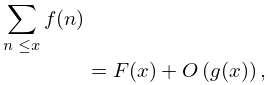
27.11.1
►where is a known function of , and represents the error, a function of smaller order than for all in some prescribed range.
…
►
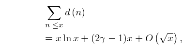
27.11.2
…
►Dirichlet’s divisor problem (unsolved as of 2022) is to determine the least number such that the error term in (27.11.2) is for all .
…
►
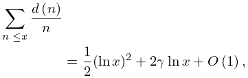
27.11.3
…
25: 3.7 Ordinary Differential Equations
…
►This converts the problem into a tridiagonal matrix problem in which the elements of the matrix are polynomials in ; compare §3.2(vi).
…
►
…
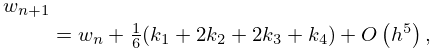
►The order estimates hold if the solution has five continuous derivatives.
…
3.7.18
…
►The order estimate holds if the solution has five continuous derivatives.
…
►
26: 18.28 Askey–Wilson Class
…
►
Duality
… ►§18.28(v) Continuous -Ultraspherical Polynomials
… ►These polynomials are also called Rogers polynomials. ►§18.28(vi) Continuous -Hermite Polynomials
… ►From Askey–Wilson to Big -Jacobi
…27: 8.11 Asymptotic Approximations and Expansions
…
►
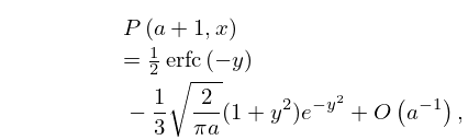
8.11.3
,
…
►
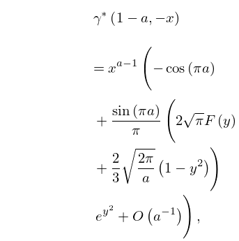
8.11.10
►
8.11.11
…
►For related expansions involving Hermite polynomials see Pagurova (1965).
…
