Watson 3F2 sum

SearchAdvancedHelp

(0.004 seconds)

1—10 of 676 matching pages

1: 34.2 Definition: $\mathit{3}j$ Symbol

§34.2 Definition: $\mathit{3}j$ Symbol

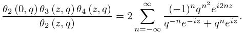
… ►The corresponding projective quantum numbers $m_1,m_2,m_3$ are given by … ►When both conditions are satisfied the $\mathit{3}j$ symbol can be expressed as the finite sum … ►where ${}_3{}^{}F_2^{}$ is defined as in §16.2. ►For alternative expressions for the $\mathit{3}j$ symbol, written either as a finite sum or as other terminating generalized hypergeometric series ${}_3{}^{}F_2^{}$ of unit argument, see Varshalovich et al. (1988, §§8.21, 8.24–8.26).

2: 20.8 Watson’s Expansions

§20.8 Watson’s Expansions

►

20.8.1 $$\frac{{\theta }_2(0,q){\theta }_3(z,q){\theta }_4(z,q)}{{\theta }_2(z,q)}=2\sum _{n=-\mathrm{\infty }}^{\mathrm{\infty }}\frac{{(-1)}^n{q}^{n^2}{\mathrm{e}}^{\mathrm{i}2nz}}{q^{-n}{\mathrm{e}}^{-\mathrm{i}z}+q^n{\mathrm{e}}^{\mathrm{i}z}}.$$

ⓘ

Symbols:

${\theta }_j(z,q)$: theta function, $\mathrm{e}$: base of natural logarithm, $\mathrm{i}$: imaginary unit, $n$: integer, $z$: complex and $q$: nome

Permalink:

http://dlmf.nist.gov/20.8.E1

Encodings:

pMML, png, TeX

See also:

Annotations for §20.8 and Ch.20

►See Watson (1935a). …

3: 16.24 Physical Applications

… ►

§16.24(i) Random Walks

►Generalized hypergeometric functions and Appell functions appear in the evaluation of the so-called Watson integrals which characterize the simplest possible lattice walks. … ►

§16.24(iii) $\mathit{3}j$, $\mathit{6}j$, and $\mathit{9}j$ Symbols

►The $\mathit{3}j$ symbols, or Clebsch–Gordan coefficients, play an important role in the decomposition of reducible representations of the rotation group into irreducible representations. They can be expressed as ${}_3{}^{}F_2^{}$ functions with unit argument. …

4: 11 Struve and Related Functions

…

5: 34.8 Approximations for Large Parameters

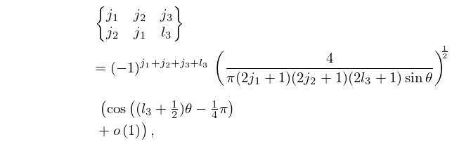
§34.8 Approximations for Large Parameters

►For large values of the parameters in the $\mathit{3}j$, $\mathit{6}j$, and $\mathit{9}j$ symbols, different asymptotic forms are obtained depending on which parameters are large. … ►

34.8.1 $j_1,j_2,j_3\gg l_3\gg 1$,

ⓘ

Symbols:

$\pi$: the ratio of the circumference of a circle to its diameter, $\cos z$: cosine function, $o\left(x\right)$: order less than, $\sin z$: sine function, : $\mathit{6}j$ symbol, $j,j_r$: non-negative integers or non-negative integers plus one half. and $l,l_r$: non-negative integers or non-negative integers plus one half.

Permalink:

http://dlmf.nist.gov/34.8.E1

Encodings:

pMML, png, TeX

See also:

Annotations for §34.8 and Ch.34

… ►Uniform approximations in terms of Airy functions for the $\mathit{3}j$ and $\mathit{6}j$ symbols are given in Schulten and Gordon (1975b). For approximations for the $\mathit{3}j$, $\mathit{6}j$, and $\mathit{9}j$ symbols with error bounds see Flude (1998), Chen et al. (1999), and Watson (1999): these references also cite earlier work.

6: 10 Bessel Functions

…

7: 10.42 Zeros

… ►The distribution of the zeros of $K_n\left(nz\right)$ in the sector $-\frac{3}{2}\pi \le \mathrm{ph}z\le \frac{1}{2}\pi$ in the cases $n=1,5,10$ is obtained on rotating Figures 10.21.2, 10.21.4, 10.21.6, respectively, through an angle $-\frac{1}{2}\pi$ so that in each case the cut lies along the positive imaginary axis. The zeros in the sector $-\frac{1}{2}\pi \le \mathrm{ph}z\le \frac{3}{2}\pi$ are their conjugates. … ►For the number of zeros of $K_{\nu }\left(z\right)$ in the sector $|\mathrm{ph}z|\le \pi$, when $\nu$ is real, see Watson (1944, pp. 511–513). …

8: 27.21 Tables

… ►Glaisher (1940) contains four tables: Table I tabulates, for all $n\le {10}^4$: (a) the canonical factorization of $n$ into powers of primes; (b) the Euler totient $\varphi \left(n\right)$; (c) the divisor function $d\left(n\right)$; (d) the sum $\sigma (n)$ of these divisors. … ►The partition function $p\left(n\right)$ is tabulated in Gupta (1935, 1937), Watson (1937), and Gupta et al. (1958). Tables of the Ramanujan function $\tau \left(n\right)$ are published in Lehmer (1943) and Watson (1949). …

9: Bibliography W

… ►

The cubic transformation of the hypergeometric function. Quart. J. Pure and Applied Math. 41, pp. 70–79.

ⓘ

External Links:

ZentralBlatt

Referenced by:

§15.8(v), §15.8(v).

Encodings:

BibTeX

►

Generating functions of class-numbers. Compositio Math. 1, pp. 39–68.

ⓘ

External Links:

ISSN 0010-437X, FullText, MathReview Entry, ZentralBlatt

Referenced by:

§20.7(v), §20.8.

Encodings:

BibTeX

►

The surface of an ellipsoid. Quart. J. Math., Oxford Ser. 6, pp. 280–287.

ⓘ

External Links:

Document, ZentralBlatt

Referenced by:

§19.33(i).

Encodings:

BibTeX

►

Two tables of partitions. Proc. London Math. Soc. (2) 42, pp. 550–556.

ⓘ

External Links:

Document, ZentralBlatt

Referenced by:

§27.21.

Encodings:

BibTeX

… ►

A table of Ramanujan’s function $\tau (n)$ . Proc. London Math. Soc. (2) 51, pp. 1–13.

ⓘ

External Links:

Document, MathReview (D. H. Lehmer), ZentralBlatt

Referenced by:

§27.21.

Encodings:

BibTeX

…

10: 20.7 Identities

… ►

§20.7(i) Sums of Squares

… ►For these and similar formulas see Lawden (1989, §1.4), Whittaker and Watson (1927, pp. 487–488), and Carlson (2011, §5). ►Also, in further development along the lines of the notations of Neville (§20.1) and of Glaisher (§22.2), the identities (20.7.6)–(20.7.9) have been recast in a more symmetric manner with respect to suffices $2,3,4$. … ►

§20.7(v) Watson’s Identities

… ►See also Carlson (2011, §3). …