Visit (-- welcom --) pharmacy buy menegatto over counterpart. ident stratege menegatto tables 100mg mills price prescription onli

SearchAdvancedHelp

(0.010 seconds)

11—20 of 516 matching pages

11: 26.18 Counting Techniques

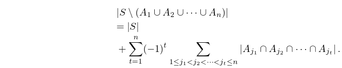
… ►Then the number of elements in the set $S\setminus (A_1\cup A_2\cup \mathrm{\cdots }\cup A_n)$ is ►

26.18.1

ⓘ

Symbols:

$\left|A\right|$: number of elements of a finite set $A$ , $\cap$: intersection, $\setminus$: set subtraction, $\cup$: union, $j$: nonnegative integer, $n$: nonnegative integer, $A_k$: subsets and $S$: set

Permalink:

http://dlmf.nist.gov/26.18.E1

Encodings:

pMML, png, TeX

See also:

Annotations for §26.18 and Ch.26

… ►Note that this is also one of the counting problems for which a formula is given in Table 26.17.1. …

12: 11.8 Analogs to Kelvin Functions

§11.8 Analogs to Kelvin Functions

►For properties of Struve functions of argument $x{\mathrm{e}}^{\pm 3\pi \mathrm{i}/4}$ see McLachlan and Meyers (1936).

13: 10.25 Definitions

… ►This equation is obtained from Bessel’s equation (10.2.1) on replacing $z$ by $\pm \mathrm{i}z$, and it has the same kinds of singularities. … ►In particular, the principal branch of $I_{\nu }\left(z\right)$ is defined in a similar way: it corresponds to the principal value of ${(\frac{1}{2}z)}^{\nu }$, is analytic in $ℂ\setminus (-\mathrm{\infty },0]$, and two-valued and discontinuous on the cut $\mathrm{ph}z=\pm \pi$. … ►The principal branch corresponds to the principal value of the square root in (10.25.3), is analytic in $ℂ\setminus (-\mathrm{\infty },0]$, and two-valued and discontinuous on the cut $\mathrm{ph}z=\pm \pi$. … ►Table 10.25.1 lists numerically satisfactory pairs of solutions (§2.7(iv)) of (10.25.1). … ►

Table 10.25.1: Numerically satisfactory pairs of solutions of the modified Bessel’s equation.

► ►►

Pair	Region
…

►

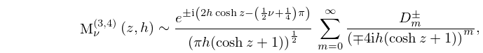
14: 28.25 Asymptotic Expansions for Large $\mathrm{\Re }z$

… ►

28.25.1 $${\mathrm{M}}_{\nu }^{(3,4)}(z,h)\sim \frac{{\mathrm{e}}^{\pm \mathrm{i}\left(2h\cosh z-\left(\frac{1}{2}\nu +\frac{1}{4}\right)\pi \right)}}{{\left(\pi h(\cosh z+1)\right)}^{\frac{1}{2}}}\sum _{m=0}^{\mathrm{\infty }}\frac{D_m^{\pm }}{{\left(\mp 4\mathrm{i}h(\cosh z+1)\right)}^m},$$

ⓘ

Symbols:

$\sim$: Poincaré asymptotic expansion, $\pi$: the ratio of the circumference of a circle to its diameter, $\mathrm{e}$: base of natural logarithm, $\cosh z$: hyperbolic cosine function, $\mathrm{i}$: imaginary unit, ${\mathrm{M}}_{\nu }^{(j)}(z,h)$: modified Mathieu function, $m$: integer, $h$: parameter, $z$: complex variable, $\nu$: complex parameter and $D_m^{\pm }$: coefficients

A&S Ref:

20.9.1 (for 3 and for integer $\nu$) 20.9.3 (for 4 and for integer $\nu$)

Referenced by:

§28.25

Permalink:

http://dlmf.nist.gov/28.25.E1

Encodings:

pMML, png, TeX

See also:

Annotations for §28.25 and Ch.28

… ►

$D_{-1}^{\pm }=0,$

►

$D_0^{\pm }=1,$

… ►

28.25.3 $$(m+1)D_{m+1}^{\pm }+\left({(m+\frac{1}{2})}^2\pm (m+\frac{1}{4})8\mathrm{i}h+2h^2-a\right)D_m^{\pm }\pm (m-\frac{1}{2})\left(8\mathrm{i}hm\right)D_{m-1}^{\pm }=0,$$ $m\ge 0$.

ⓘ

Symbols:

$\mathrm{i}$: imaginary unit, $m$: integer, $h$: parameter, $a$: parameter and $D_m^{\pm }$: coefficients

A&S Ref:

20.9.2 (for $+$) 20.9.4 (for $-$)

Permalink:

http://dlmf.nist.gov/28.25.E3

Encodings:

pMML, png, TeX

See also:

Annotations for §28.25 and Ch.28

…

15: 4.13 Lambert $W$-Function

… ►The decreasing solution can be identified as $W_{\pm 1}\left(x\mp 0\mathrm{i}\right)$. …$W_0\left(z\right)$ is a single-valued analytic function on $ℂ\setminus (-\mathrm{\infty },-{\mathrm{e}}^{-1}]$, real-valued when $z>-{\mathrm{e}}^{-1}$, and has a square root branch point at $z=-{\mathrm{e}}^{-1}$. …The other branches $W_k\left(z\right)$ are single-valued analytic functions on $ℂ\setminus (-\mathrm{\infty },0]$, have a logarithmic branch point at $z=0$, and, in the case $k=\pm 1$, have a square root branch point at $z=-{\mathrm{e}}^{-1}\mp 0\mathrm{i}$ respectively. … ►and has several advantages over the Lambert $W$-function (see Lawrence et al. (2012)), and the tree $T$-function $T\left(z\right)=-W\left(-z\right)$, which is a solution of … ►where $t\ge 0$ for $W_0$, $t\le 0$ for $W_{\pm 1}$ on the relevant branch cuts, …

16: 22.9 Cyclic Identities

§22.9 Cyclic Identities

… ►

§22.9(ii) Typical Identities of Rank 2

… ► ►

§22.9(iii) Typical Identities of Rank 3

… ►

17: 7.23 Tables

§7.23 Tables

… ►This section lists relevant tables that appeared later. … ►

Zhang and Jin (1996, pp. 637, 639) includes $(2/\sqrt{\pi }){\mathrm{e}}^{-x^2}$, $\mathrm{erf}x$, $x=0(.02)1(.04)3$, 8D; $C\left(x\right)$, $S\left(x\right)$, $x=0(.2)10(2)100(100)500$, 8D.

… ►

Zhang and Jin (1996, pp. 638, 640–641) includes the real and imaginary parts of $\mathrm{erf}z$, $x\in [0,5]$, $y=0.5(.5)3$, 7D and 8D, respectively; the real and imaginary parts of ${\int }_x^{\mathrm{\infty }}{\mathrm{e}}^{\pm \mathrm{i}{t}^2}dt$, $(1/\sqrt{\pi }){\mathrm{e}}^{\mp \mathrm{i}(x^2+(\pi /4))}{\int }_x^{\mathrm{\infty }}{\mathrm{e}}^{\pm \mathrm{i}{t}^2}dt$, $x=0(.5)20(1)25$, 8D, together with the corresponding modulus and phase to 8D and 6D (degrees), respectively.

… ►

Fettis et al. (1973) gives the first 100 zeros of $\mathrm{erf}z$ and $w\left(z\right)$ (the table on page 406 of this reference is for $w\left(z\right)$, not for $\mathrm{erfc}z$), 11S.

…

18: Charles W. Clark

… ►He has been a Visiting Fellow at the Australian National University, a Dr. Lee Fellow at Christ Church College of the University of Oxford, and Visiting Professor at the National University of Singapore. ►Clark received the R&D 100 Award, Distinguished Presidential Rank Award of the U. …

19: 6.4 Analytic Continuation

… ►

6.4.3 $$E_1\left(z{\mathrm{e}}^{\pm \pi \mathrm{i}}\right)=\mathrm{Ein}\left(-z\right)-\ln z-\gamma \mp \pi \mathrm{i},$$ $|\mathrm{ph}z|\le \pi$.

ⓘ

Symbols:

$\gamma$: Euler’s constant, $\pi$: the ratio of the circumference of a circle to its diameter, $\mathrm{Ein}\left(z\right)$: complementary exponential integral, $\mathrm{e}$: base of natural logarithm, $E_1\left(z\right)$: exponential integral, $\mathrm{i}$: imaginary unit, $\ln z$: principal branch of logarithm function, $\mathrm{ph}$: phase and $z$: complex variable

Referenced by:

§6.4

Permalink:

http://dlmf.nist.gov/6.4.E3

Encodings:

pMML, png, TeX

See also:

Annotations for §6.4 and Ch.6

… ►

6.4.4 $$\mathrm{Ci}\left(z{\mathrm{e}}^{\pm \pi \mathrm{i}}\right)=\pm \pi \mathrm{i}+\mathrm{Ci}\left(z\right),$$

ⓘ

Symbols:

$\pi$: the ratio of the circumference of a circle to its diameter, $\mathrm{Ci}\left(z\right)$: cosine integral, $\mathrm{e}$: base of natural logarithm, $\mathrm{i}$: imaginary unit and $z$: complex variable

Referenced by:

§6.4

Permalink:

http://dlmf.nist.gov/6.4.E4

Encodings:

pMML, png, TeX

See also:

Annotations for §6.4 and Ch.6

►

6.4.5 $$\mathrm{Chi}\left(z{\mathrm{e}}^{\pm \pi \mathrm{i}}\right)=\pm \pi \mathrm{i}+\mathrm{Chi}\left(z\right),$$

ⓘ

Symbols:

$\pi$: the ratio of the circumference of a circle to its diameter, $\mathrm{e}$: base of natural logarithm, $\mathrm{Chi}\left(z\right)$: hyperbolic cosine integral, $\mathrm{i}$: imaginary unit and $z$: complex variable

Referenced by:

§6.4

Permalink:

http://dlmf.nist.gov/6.4.E5

Encodings:

pMML, png, TeX

See also:

Annotations for §6.4 and Ch.6

►

6.4.6 $$\mathrm{f}\left(z{\mathrm{e}}^{\pm \pi \mathrm{i}}\right)=\pi {\mathrm{e}}^{\mp \mathrm{i}z}-\mathrm{f}\left(z\right),$$

ⓘ

Symbols:

$\pi$: the ratio of the circumference of a circle to its diameter, $\mathrm{e}$: base of natural logarithm, $\mathrm{i}$: imaginary unit, $\mathrm{f}\left(z\right)$: auxiliary function for sine and cosine integrals and $z$: complex variable

Referenced by:

§6.12(ii), §6.4

Permalink:

http://dlmf.nist.gov/6.4.E6

Encodings:

pMML, png, TeX

See also:

Annotations for §6.4 and Ch.6

►

6.4.7 $$\mathrm{g}\left(z{\mathrm{e}}^{\pm \pi \mathrm{i}}\right)=\mp \pi \mathrm{i}{\mathrm{e}}^{\mp \mathrm{i}z}+\mathrm{g}\left(z\right).$$

ⓘ

Symbols:

$\pi$: the ratio of the circumference of a circle to its diameter, $\mathrm{e}$: base of natural logarithm, $\mathrm{i}$: imaginary unit, $\mathrm{g}\left(z\right)$: auxiliary function for sine and cosine integrals and $z$: complex variable

Referenced by:

§6.12(ii), §6.4

Permalink:

http://dlmf.nist.gov/6.4.E7

Encodings:

pMML, png, TeX

See also:

Annotations for §6.4 and Ch.6

…

20: 10.20 Uniform Asymptotic Expansions for Large Order

… ►For numerical tables of $\zeta =\zeta (z)$, ${(4\zeta /(1-z^2))}^{\frac{1}{4}}$ and $A_k(\zeta )$, $B_k(\zeta )$, $C_k(\zeta )$, and $D_k(\zeta )$ see Olver (1962, pp. 28–42). … ►

10.20.17 $$z=\pm {(\tau \coth \tau -{\tau }^2)}^{\frac{1}{2}}\pm \mathrm{i}{({\tau }^2-\tau \tanh \tau )}^{\frac{1}{2}},$$ $0\le \tau \le {\tau }_0$,

ⓘ

Symbols:

$\coth z$: hyperbolic cotangent function, $\tanh z$: hyperbolic tangent function, $\mathrm{i}$: imaginary unit and $z$: complex variable

Permalink:

http://dlmf.nist.gov/10.20.E17

Encodings:

pMML, png, TeX

See also:

Annotations for §10.20(ii), §10.20 and Ch.10

… ►The points $P_1,P_2$ where these curves intersect the imaginary axis are $\pm \mathrm{i}c$, where … ►

►►

Figure 10.20.1: $z$-plane. $P_1$ and $P_2$ are the points $\pm \mathrm{i}c$. … Magnify

►

►►

Figure 10.20.2: $\zeta$-plane. $E_1$ and $E_2$ are the points ${\mathrm{e}}^{\mp \pi \mathrm{i}/3}{(3\pi /2)}^{2/3}.$ Magnify

…