Legendre functions on the cut

SearchAdvancedHelp

(0.003 seconds)

11—19 of 19 matching pages

11: 30.16 Methods of Computation

… ►

30.16.9 $${\mathrm{𝖯𝗌}}_n^m(x,{\gamma }^2)=\underset{d\to \mathrm{\infty }}{lim}\sum _{j=1}^d{(-1)}^{j-p}{e}_{j,d}{𝖯}_{n+2(j-p)}^m\left(x\right).$$

ⓘ

Symbols:

: Ferrers function of the first kind, ${\mathrm{𝖯𝗌}}_n^m(x,{\gamma }^2)$: spheroidal wave function of the first kind, $x$: real variable, $m$: nonnegative integer, $n\ge m$: integer degree, $d$: dimension and ${\gamma }^2$: real parameter

Permalink:

http://dlmf.nist.gov/30.16.E9

Encodings:

pMML, png, TeX

See also:

Annotations for §30.16(ii), §30.16 and Ch.30

…

12: 14.21 Definitions and Basic Properties

… ►When $z$ is complex $P_{\nu }^{\pm \mu }\left(z\right)$, $Q_{\nu }^{\mu }\left(z\right)$, and ${𝑸}_{\nu }^{\mu }\left(z\right)$ are defined by (14.3.6)–(14.3.10) with $x$ replaced by $z$: the principal branches are obtained by taking the principal values of all the multivalued functions appearing in these representations when $z\in (1,\mathrm{\infty })$, and by continuity elsewhere in the $z$-plane with a cut along the interval $(-\mathrm{\infty },1]$; compare §4.2(i). …

13: 14.24 Analytic Continuation

§14.24 Analytic Continuation

►Let $s$ be an arbitrary integer, and $P_{\nu }^{-\mu }\left(z{\mathrm{e}}^{s\pi \mathrm{i}}\right)$ and ${𝑸}_{\nu }^{\mu }\left(z{\mathrm{e}}^{s\pi \mathrm{i}}\right)$ denote the branches obtained from the principal branches by making $\frac{1}{2}s$ circuits, in the positive sense, of the ellipse having $\pm 1$ as foci and passing through $z$. … ►Next, let $P_{\nu ,s}^{-\mu }\left(z\right)$ and ${𝑸}_{\nu ,s}^{\mu }\left(z\right)$ denote the branches obtained from the principal branches by encircling the branch point $1$ (but not the branch point $-1$) $s$ times in the positive sense. … ►For fixed $z$, other than $\pm 1$ or $\mathrm{\infty }$, each branch of $P_{\nu }^{-\mu }\left(z\right)$ and ${𝑸}_{\nu }^{\mu }\left(z\right)$ is an entire function of each parameter $\nu$ and $\mu$. ►The behavior of $P_{\nu }^{-\mu }\left(z\right)$ and ${𝑸}_{\nu }^{\mu }\left(z\right)$ as $z\to -1$ from the left on the upper or lower side of the cut from $-\mathrm{\infty }$ to $1$ can be deduced from (14.8.7)–(14.8.11), combined with (14.24.1) and (14.24.2) with $s=\pm 1$.

14: 10.43 Integrals

… ►

§10.43(iii) Fractional Integrals

… ►For the second equation there is a cut in the $a$-plane along the interval $[0,1]$, and all quantities assume their principal values (§4.2(i)). For the Ferrers function $𝖯$ and the associated Legendre function $P$, see §§14.3(i) and 14.21(i). … … ►The Kontorovich–Lebedev transform of a function $g(x)$ is defined as …

15: 19.2 Definitions

… ►

§19.2(ii) Legendre’s Integrals

… ►Legendre’s complementary complete elliptic integrals are defined via … ►Bulirsch’s integrals are linear combinations of Legendre’s integrals that are chosen to facilitate computational application of Bartky’s transformation (Bartky (1938)). … ►Lastly, corresponding to Legendre’s incomplete integral of the third kind we have … ►

§19.2(iv) A Related Function: $R_C(x,y)$

…

16: 30.1 Special Notation

… ►The main functions treated in this chapter are the eigenvalues ${\lambda }_n^m\left({\gamma }^2\right)$ and the spheroidal wave functions ${\mathrm{𝖯𝗌}}_n^m(x,{\gamma }^2)$, ${\mathrm{𝖰𝗌}}_n^m(x,{\gamma }^2)$, ${\mathrm{𝑃𝑠}}_n^m(z,{\gamma }^2)$, ${\mathrm{𝑄𝑠}}_n^m(z,{\gamma }^2)$, and $S_n^{m(j)}(z,\gamma )$, $j=1,2,3,4$. …Meixner and Schäfke (1954) use $\mathrm{ps}$, $\mathrm{qs}$, $\mathrm{Ps}$, $\mathrm{Qs}$ for $\mathrm{𝖯𝗌}$, $\mathrm{𝖰𝗌}$, $\mathrm{𝑃𝑠}$, $\mathrm{𝑄𝑠}$, respectively. ►

Other Notations

►Flammer (1957) and Abramowitz and Stegun (1964) use ${\lambda }_{mn}(\gamma )$ for ${\lambda }_n^m\left({\gamma }^2\right)+{\gamma }^2$, $R_{mn}^{(j)}(\gamma ,z)$ for $S_n^{m(j)}(z,\gamma )$, and …

17: 19.3 Graphics

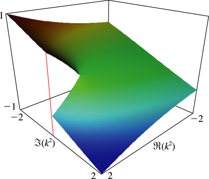
§19.3 Graphics

… ►See Figures 19.3.1–19.3.6 for complete and incomplete Legendre’s elliptic integrals. … ►In Figures 19.3.7 and 19.3.8 for complete Legendre’s elliptic integrals with complex arguments, height corresponds to the absolute value of the function and color to the phase. … ►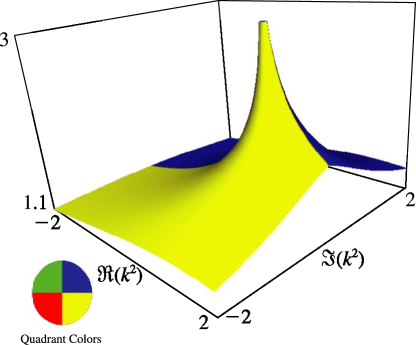

►

►

Figure 19.3.7: $K\left(k\right)$ as a function of complex $k^2$ for $-2\le \mathrm{\Re }\left(k^2\right)\le 2$, $-2\le \mathrm{\Im }\left(k^2\right)\le 2$. There is a branch cut where . Magnify 3D Help

… ►

►

►

Figure 19.3.12: $\mathrm{\Im }\left(E\left(k\right)\right)$ as a function of complex $k^2$ for $-2\le \mathrm{\Re }\left(k^2\right)\le 2$, $-2\le \mathrm{\Im }\left(k^2\right)\le 2$. … Magnify 3D Help

18: 30.6 Functions of Complex Argument

§30.6 Functions of Complex Argument

►The solutions … ►

Relations to Associated Legendre Functions

… ►

30.6.5 $${\mathrm{𝑄𝑠}}_n^m(x\pm \mathrm{i}0,{\gamma }^2)={(\mp \mathrm{i})}^m\left({\mathrm{𝖰𝗌}}_n^m(x,{\gamma }^2)\mp \frac{1}{2}\mathrm{i}\pi {\mathrm{𝖯𝗌}}_n^m(x,{\gamma }^2)\right).$$

ⓘ

Symbols:

$\pi$: the ratio of the circumference of a circle to its diameter, $\mathrm{i}$: imaginary unit, ${\mathrm{𝑄𝑠}}_n^m(z,{\gamma }^2)$: spheroidal wave function of complex argument, ${\mathrm{𝖯𝗌}}_n^m(x,{\gamma }^2)$: spheroidal wave function of the first kind, ${\mathrm{𝖰𝗌}}_n^m(x,{\gamma }^2)$: spheroidal wave function of the second kind, $x$: real variable, $m$: nonnegative integer, $n\ge m$: integer degree and ${\gamma }^2$: real parameter

Permalink:

http://dlmf.nist.gov/30.6.E5

Encodings:

pMML, png, TeX

See also:

Annotations for §30.6, §30.6 and Ch.30

… ►

19: 2.10 Sums and Sequences

… ►Then … ►

§2.10(iii) Asymptotic Expansions of Entire Functions

… ►

Example

►Let $\alpha$ be a constant in $(0,2\pi )$ and $P_n$ denote the Legendre polynomial of degree $n$. …Here the branch of ${\left({\mathrm{e}}^{-\mathrm{i}\alpha }-z\right)}^{-1/2}$ is continuous in the $z$-plane cut along the outward-drawn ray through $z={\mathrm{e}}^{-\mathrm{i}\alpha }$ and equals ${\mathrm{e}}^{\mathrm{i}\alpha /2}$ at $z=0$. …