.世界杯直播频道cctv5回放_『wn4.com_』国足参加过世界杯吗_w6n2c9o_2022年11月29日22时50分34秒_k6imqu2oe
(0.006 seconds)
21—30 of 786 matching pages
21: 16.4 Argument Unity
…
►The function is well-poised if
…It is very well-poised if it is well-poised and .
…
►The function with argument unity and general values of the parameters is discussed in Bühring (1992).
…
►For generalizations involving functions see Kim et al. (2013).
…
►Transformations for both balanced and very well-poised are included in Bailey (1964, pp. 56–63).
…
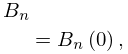
22: 24.2 Definitions and Generating Functions
23: 21.1 Special Notation
…
►
►
…
| positive integers. | |
| … | |
| th element of vector . | |
| … | |
| Transpose of . | |
| … | |
| . | |
| … | |
| set of all elements of the form “”. | |
| set of all elements of , modulo elements of . Thus two elements of are equivalent if they are both in and their difference is in . (For an example see §20.12(ii).) | |
| … | |
24: 17.7 Special Cases of Higher Functions
…
►
§17.7(i) Functions
►-Analog of Bailey’s Sum
… ►-Analog of Gauss’s Sum
… ►-Analog of Dixon’s Sum
… ►where are arbitrary nonnegative integers. …25: 28.6 Expansions for Small
…
►Leading terms of the power series for and for are:
…
►The coefficients of the power series of , and also , are the same until the terms in and , respectively.
…
►Numerical values of the radii of convergence of the power series (28.6.1)–(28.6.14) for are given in Table 28.6.1.
Here for , for , and for and .
…
►
§28.6(ii) Functions and
…26: 3.1 Arithmetics and Error Measures
…
►with and all allowable choices of , , , and .
…
►Let with and .
…The integers , , and are characteristics of the machine.
…
►The respective machine precisions are , and .
…
►
, and
…
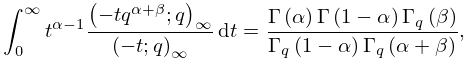
27: 17.13 Integrals
28: 24.20 Tables
…
►Abramowitz and Stegun (1964, Chapter 23) includes exact values of , , ; , , , , 20D; , , 18D.
►Wagstaff (1978) gives complete prime factorizations of and for and , respectively.
…
►For information on tables published before 1961 see Fletcher et al. (1962, v. 1, §4) and Lebedev and Fedorova (1960, Chapters 11 and 14).
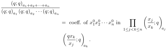
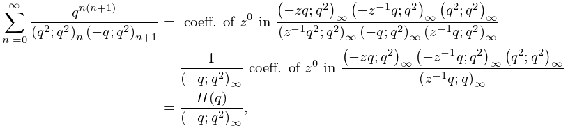
29: 17.14 Constant Term Identities
30: 24.19 Methods of Computation
…
►Equations (24.5.3) and (24.5.4) enable and to be computed by recurrence.
…For example, the tangent numbers can be generated by simple recurrence relations obtained from (24.15.3), then (24.15.4) is applied.
…
►If denotes the right-hand side of (24.19.1) but with the second product taken only for , then for .
…
►For algorithms for computing , , , and see Spanier and Oldham (1987, pp. 37, 41, 171, and 179–180).
►
