two%20or%20more%20variables

SearchAdvancedHelp

(0.003 seconds)

21—30 of 31 matching pages

21: 20.10 Integrals

…

22: Bibliography N

… ►

On an integral transform involving a class of Mathieu functions. SIAM J. Math. Anal. 20 (6), pp. 1500–1513.

ⓘ

External Links:

ISSN 0036-1410, Document, MathReview (K. C. Gupta), ZentralBlatt

Referenced by:

§28.26(ii).

Encodings:

BibTeX

… ►

Reduction and evaluation of elliptic integrals. Math. Comp. 20 (94), pp. 223–231.

ⓘ

External Links:

FullText, MathReview (I. A. Stegun), ZentralBlatt

Referenced by:

§19.37(iv).

Encodings:

BibTeX

… ►

Proofs of two conjectures on the real zeros of the cylinder and Airy functions. SIAM J. Math. Anal. 53 (4), pp. 4328–4349.

ⓘ

External Links:

ISSN 0036-1410, Document, Link, MathReview (José Luis López), ZentralBlatt

Referenced by:

(10.18.17), (10.18.18), §10.18(iii), (9.8.22), (9.8.23), §9.8(iv), Erratum (V1.1.8) for Section 9.8(iv), Erratum (V1.1.8) for Section 10.18(iii).

Encodings:

BibTeX

… ►

A table of integrals of the error functions. J. Res. Nat. Bur. Standards Sect B. 73B, pp. 1–20.

ⓘ

Notes:

See for additions and corrections same journal, Sect. B 75, 149–163 (1975)

External Links:

MathReview, ZentralBlatt

Referenced by:

§7.14(iii), §7.21, §7.7(iii).

Encodings:

BibTeX

…

23: Bibliography W

… ►

The Nahm equations, finite-gap potentials and Lamé functions. J. Phys. A 20 (10), pp. 2679–2683.

ⓘ

External Links:

ISSN 0305-4470, Document, MathReview (James M. D’Archangelo), ZentralBlatt

Referenced by:

§29.19(ii).

Encodings:

BibTeX

… ►

Two tables of partitions. Proc. London Math. Soc. (2) 42, pp. 550–556.

ⓘ

External Links:

Document, ZentralBlatt

Referenced by:

§27.21.

Encodings:

BibTeX

… ►

An asymptotic expansion of $W_{k,m}(z)$ with large variable and parameters. Math. Comp. 27 (122), pp. 429–436.

ⓘ

External Links:

FullText, Document, MathReview (J. A. Donaldson), ZentralBlatt

Referenced by:

§13.19.

Encodings:

BibTeX

… ►

Concerning two series for the gamma function. Math. Comp. 22 (103), pp. 617–626.

ⓘ

External Links:

FullText, Document, MathReview (I. A. Stegun), ZentralBlatt

Referenced by:

§5.11(i), §5.7(i), §5.7(i).

Encodings:

BibTeX

… ►

Spin-spin correlation functions for the two-dimensional Ising model: Exact theory in the scaling region. Phys. Rev. B 13, pp. 316–374.

ⓘ

External Links:

Document, Link

Referenced by:

§32.16, §32.16.

Encodings:

BibTeX

…

24: 26.13 Permutations: Cycle Notation

… ►A transposition is a permutation that consists of a single cycle of length two. An adjacent transposition is a transposition of two consecutive integers. A permutation that consists of a single cycle of length $k$ can be written as the composition of $k-1$ two-cycles (read from right to left): …

25: 22.3 Graphics

… ►

§22.3(i) Real Variables: Line Graphs

… ►

§22.3(ii) Real Variables: Surfaces

… ►

►

►

Figure 22.3.13: $\mathrm{sn}(x,k)$ for $k=1-{\mathrm{e}}^{-n}$, $n=0$ to 20, $-5\pi \le x\le 5\pi$. Magnify 3D Help

… ►

§22.3(iii) Complex $z$; Real $k$

… ►

►►

Figure 22.3.28: Density plot of $|\mathrm{sn}(20,k)|$ as a function of complex $k^2$, $-10\le \mathrm{\Re }\left(k^2\right)\le 20$, $-10\le \mathrm{\Im }\left(k^2\right)\le 10$. … Magnify

…

26: 3.8 Nonlinear Equations

… ►(More precisely, $p$ is the largest of the possible set of indices for (3.8.3).) … ►If with , then the interval $[a,b]$ contains one or more zeros of $f$. … ►This example illustrates the fact that the method succeeds even if the two zeros of the wanted quadratic factor are real and the same. … ►Consider $x=20$ and $j=19$. We have $p^{\prime }(20)=19!$ and $a_{19}=1+2+\mathrm{\cdots }+20=210$. …

27: Bibliography P

… ►

On two-sided estimates, uniform with respect to the real argument and index, for modified Bessel functions. Mat. Zametki 65 (5), pp. 681–692 (Russian).

ⓘ

Notes:

English translation in Math. Notes 65 (1999) pp. 571-581.

External Links:

ISSN 0025-567X, Document, MathReview (Boro Döring), ZentralBlatt

Referenced by:

§10.37.

Encodings:

BibTeX

… ►

The asymptotic behaviour of Pearcey’s integral for complex variables. Proc. Roy. Soc. London Ser. A 432 (1886), pp. 391–426.

ⓘ

External Links:

ISSN 0962-8444, Document, Link, MathReview (J. S. Joel), ZentralBlatt

Referenced by:

§36.12(i).

Encodings:

BibTeX

… ►

Automatic computation of Bessel function integrals. Comput. Phys. Comm. 25 (3), pp. 289–295.

ⓘ

Notes:

Double-precision Fortran, maximum accuracy 20S.

External Links:

ISSN 0010-4655, Document, Code

Referenced by:

6th item.

Encodings:

BibTeX

… ►

Remarks on computing the probability integral in one and two dimensions. In Proceedings of the Berkeley Symposium on Mathematical Statistics and Probability, 1945, 1946, pp. 63–78.

ⓘ

External Links:

MathReview (L. A. Aroian), ZentralBlatt

Referenced by:

(7.8.8), §7.8, Erratum (V1.0.17) for Equation (7.8.8).

Encodings:

BibTeX

… ►

Integrals and Series: More Special Functions, Vol. 3. Gordon and Breach Science Publishers, New York.

ⓘ

Notes:

Translated from the Russian by G. G. Gould. Table erratum Math. Comp. v. 65 (1996), no. 215, p. 1384.

External Links:

ISBN 2-88124-682-6, MathReview, ZentralBlatt

Referenced by:

§1.14(viii), §1.4(iv), §11.10(x), §11.10(x), §11.7(v), §11.7(v), §11.9(iv), §13.10(vi), §13.11, §13.23(v), §13.24(ii), (13.6.11_1), (13.6.11_2), §14.17(i), §14.17(iv), §14.18(iv), §14.20(x), §15.14, §15.15, §15.4(i), §16.10, §16.20, §16.20, §16.5, §19.13(i), §19.13(i), §19.13(ii), §20.10(iii), §23.14, §24.13(iii), §24.14(iii), §25.11(ix), §25.11(xi), §25.12(ii), §28.10(iii), §28.28(v), §9.10(ix), §9.11(v).

Encodings:

BibTeX

…

28: 25.5 Integral Representations

… ►

25.5.1 $$\zeta \left(s\right)=\frac{1}{\mathrm{\Gamma }\left(s\right)}{\int }_0^{\mathrm{\infty }}\frac{x^{s-1}}{{\mathrm{e}}^x-1}dx,$$ $\mathrm{\Re }s>1$.

ⓘ

Symbols:

$\mathrm{\Gamma }\left(z\right)$: gamma function, $\zeta \left(s\right)$: Riemann zeta function, $dx$: differential of $x$ , $\mathrm{e}$: base of natural logarithm, $\int$: integral, $\mathrm{\Re }$: real part, $x$: real variable and $s$: complex variable

Keywords:

improper integral, integral representation

Source:

Erdélyi et al. (1953a, (1.12.4), p. 32)

A&S Ref:

23.2.7

Referenced by:

§25.12(ii), (25.5.2), (25.5.6)

Permalink:

http://dlmf.nist.gov/25.5.E1

Encodings:

pMML, png, TeX

See also:

Annotations for §25.5(i), §25.5 and Ch.25

►

25.5.2 $$\zeta \left(s\right)=\frac{1}{\mathrm{\Gamma }\left(s+1\right)}{\int }_0^{\mathrm{\infty }}\frac{{\mathrm{e}}^x{x}^s}{{({\mathrm{e}}^x-1)}^2}dx,$$ $\mathrm{\Re }s>1$.

ⓘ

Symbols:

$\mathrm{\Gamma }\left(z\right)$: gamma function, $\zeta \left(s\right)$: Riemann zeta function, $dx$: differential of $x$ , $\mathrm{e}$: base of natural logarithm, $\int$: integral, $\mathrm{\Re }$: real part, $x$: real variable and $s$: complex variable

Keywords:

improper integral, integral representation

Proof sketch:

Derivable from (25.5.1) by integration by parts.

Permalink:

http://dlmf.nist.gov/25.5.E2

Encodings:

pMML, png, TeX

See also:

Annotations for §25.5(i), §25.5 and Ch.25

►

25.5.3 $$\zeta \left(s\right)=\frac{1}{(1-2^{1-s})\mathrm{\Gamma }\left(s\right)}{\int }_0^{\mathrm{\infty }}\frac{x^{s-1}}{{\mathrm{e}}^x+1}dx,$$ $\mathrm{\Re }s>0$.

ⓘ

Symbols:

$\mathrm{\Gamma }\left(z\right)$: gamma function, $\zeta \left(s\right)$: Riemann zeta function, $dx$: differential of $x$ , $\mathrm{e}$: base of natural logarithm, $\int$: integral, $\mathrm{\Re }$: real part, $x$: real variable and $s$: complex variable

Keywords:

improper integral, integral representation

Source:

Erdélyi et al. (1953a, (1.12.5), p. 32)

A&S Ref:

23.2.8

Referenced by:

(25.5.4)

Permalink:

http://dlmf.nist.gov/25.5.E3

Encodings:

pMML, png, TeX

See also:

Annotations for §25.5(i), §25.5 and Ch.25

… ►

25.5.5 $$\zeta \left(s\right)=-s{\int }_0^{\mathrm{\infty }}\frac{x-\lfloor x\rfloor -\frac{1}{2}}{x^{s+1}}dx,$$ .

ⓘ

Symbols:

$\zeta \left(s\right)$: Riemann zeta function, $dx$: differential of $x$ , $\lfloor x\rfloor$: floor of $x$ , $\int$: integral, $\mathrm{\Re }$: real part, $x$: real variable and $s$: complex variable

Keywords:

improper integral, integral representation

Source:

Titchmarsh (1986b, (2.1.6), p. 15)

Permalink:

http://dlmf.nist.gov/25.5.E5

Encodings:

pMML, png, TeX

See also:

Annotations for §25.5(i), §25.5 and Ch.25

… ►

25.5.7 $$\zeta \left(s\right)=\frac{1}{2}+\frac{1}{s-1}+\sum _{m=1}^n\frac{B_{2m}}{(2m)!}{\left(s\right)}_{2m-1}+\frac{1}{\mathrm{\Gamma }\left(s\right)}{\int }_0^{\mathrm{\infty }}\left(\frac{1}{{\mathrm{e}}^x-1}-\frac{1}{x}+\frac{1}{2}-\sum _{m=1}^n\frac{B_{2m}}{(2m)!}{x}^{2m-1}\right)\frac{x^{s-1}}{{\mathrm{e}}^x}dx,$$ $\mathrm{\Re }s>-(2n+1)$, $n=1,2,3,\mathrm{\dots }$.

ⓘ

Symbols:

$B_n$: Bernoulli numbers, $O\left(x\right)$: order not exceeding, $\mathrm{\Gamma }\left(z\right)$: gamma function, ${\left(a\right)}_n$: Pochhammer’s symbol (or shifted factorial), $\zeta \left(s\right)$: Riemann zeta function, $dx$: differential of $x$ , $\mathrm{e}$: base of natural logarithm, $!$: factorial (as in $n!$), $\int$: integral, $\mathrm{\Re }$: real part, $m$: nonnegative integer, $n$: nonnegative integer, $x$: real variable and $s$: complex variable

Keywords:

improper integral, integral representation

Proof sketch:

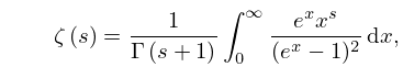
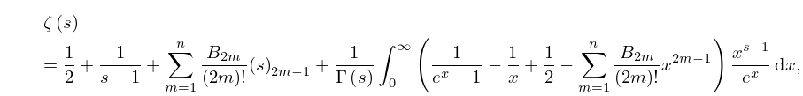
Derivable from (25.5.6) by adding and subtracting ${\sum }_{m=1}^n{B}_{2m}{x}^{2m-1}/(2m)!$ in the integrand, using (5.2.1), (5.2.5), and recognizing that ${({\mathrm{e}}^x-1)}^{-1}-x^{-1}+1/2-{\sum }_{m=1}^n{B}_{2m}{x}^{2m-1}/(2m)!=O\left(x^{2n+1}\right)$ as $x\to 0$, demonstrating the region of convergence.

Referenced by:

Erratum (V1.0.9) for Chapters 7, 25

Permalink:

http://dlmf.nist.gov/25.5.E7

Encodings:

pMML, png, TeX

Notational Change (effective with 1.0.9):

We have rewritten the original summation ${\sum }_{m=1}^n\frac{B_{2m}}{(2m)!}\frac{\mathrm{\Gamma }\left(s+2m-1\right)}{\mathrm{\Gamma }\left(s\right)}$ more concisely as ${\sum }_{m=1}^n\frac{B_{2m}}{(2m)!}{\left(s\right)}_{2m-1}$ using the Pochhammer symbol.

See also:

Annotations for §25.5(i), §25.5 and Ch.25

…

29: 3.4 Differentiation

… ►

Two-Point Formula

… ►

$$B_{-2}^5=\frac{1}{120}(6-10t-15t^2+20t^3-5t^4),$$

… ►

$$B_{-3}^6=-\frac{1}{720}(12-8t-45t^2+20t^3+15t^4-6t^5),$$

►

$$B_{-2}^6=\frac{1}{60}(9-9t-30t^2+20t^3+5t^4-3t^5),$$

… ►

$$B_2^6=-\frac{1}{60}(9+9t-30t^2-20t^3+5t^4+3t^5),$$

…

30: Bibliography O

… ►

Summing one- and two-dimensional series related to the Euler series. J. Comput. Appl. Math. 98 (2), pp. 245–271.

ⓘ

External Links:

ISSN 0377-0427, Document, MathReview (Boris Petrovich Osilenker), ZentralBlatt

Referenced by:

§25.8.

Encodings:

BibTeX

… ►

An error analysis of the modified Clenshaw method for evaluating Chebyshev and Fourier series. J. Inst. Math. Appl. 20 (3), pp. 379–391.

ⓘ

External Links:

Document, MathReview (David L. Elliott), ZentralBlatt

Referenced by:

§3.11(ii).

Encodings:

BibTeX

… ►

Second-order linear differential equations with two turning points. Philos. Trans. Roy. Soc. London Ser. A 278, pp. 137–174.

ⓘ

External Links:

FullText, MathReview (P. F. Hsieh), ZentralBlatt

Referenced by:

§2.8(vi).

Encodings:

BibTeX

… ►

Improved error bounds for second-order differential equations with two turning points. J. Res. Nat. Bur. Standards Sect. B 80B (4), pp. 437–440.

ⓘ

External Links:

MathReview (Peter Deuflhard), ZentralBlatt

Referenced by:

§2.8(vi).

Encodings:

BibTeX

… ►

Iterative Solution of Nonlinear Equations in Several Variables. Academic Press, New York.

ⓘ

Notes:

Reprinted in 2000 by the Society for Industrial and Applied Mathematics (SIAM), Philadelphia, Pennsylvania

External Links:

MathReview (J. F. Traub), ZentralBlatt (Nelli Dimitrova (Sofia))

Referenced by:

§3.8(vii).

Encodings:

BibTeX

…