extended complex plane

SearchAdvancedHelp

(0.003 seconds)

11—20 of 28 matching pages

11: 25.16 Mathematical Applications

… ►

25.16.5 $$H\left(s\right)=\sum _{n=1}^{\mathrm{\infty }}\frac{H_n}{n^s},$$

ⓘ

Symbols:

$H\left(s\right)$: Euler sums, $H_n$: harmonic number, $n$: nonnegative integer, $s$: complex variable and $h(n)$: harmonic number

Keywords:

Euler sum, infinite series, series representation

Source:

Apostol and Vu (1984, p. 85)

Referenced by:

Erratum (V1.1.4) for Notation

Permalink:

http://dlmf.nist.gov/25.16.E5

Encodings:

pMML, png, TeX

Notation (effective with 1.1.4):

The notation previously used for the harmonic number $h(n)$ has been replaced to be $H_n$.

Suggested 2021-08-23 by Gergő Nemes

See also:

Annotations for §25.16(ii), §25.16 and Ch.25

… ► $H\left(s\right)$ is analytic for $\mathrm{\Re }s>1$, and can be extended meromorphically into the half-plane $\mathrm{\Re }s>-2k$ for every positive integer $k$ by use of the relations … ►

25.16.9 $$H\left(a\right)=\frac{a+2}{2}\zeta \left(a+1\right)-\frac{1}{2}\sum _{r=1}^{a-2}\zeta \left(r+1\right)\zeta \left(a-r\right),$$ $a=2,3,4,\mathrm{\dots }$.

ⓘ

Symbols:

$H\left(s\right)$: Euler sums, $\zeta \left(s\right)$: Riemann zeta function and $a$: real or complex parameter

Source:

Apostol and Vu (1984, (12), p. 92)

Referenced by:

(25.16.8)

Permalink:

http://dlmf.nist.gov/25.16.E9

Encodings:

pMML, png, TeX

See also:

Annotations for §25.16(ii), §25.16 and Ch.25

… ►

25.16.11 $$H(s,z)=\sum _{n=1}^{\mathrm{\infty }}\frac{1}{n^s}\sum _{m=1}^n\frac{1}{m^z},$$ $\mathrm{\Re }\left(s+z\right)>1$,

ⓘ

Symbols:

$H(s,z)$: generalized Euler sums, $\mathrm{\Re }$: real part, $m$: nonnegative integer, $n$: nonnegative integer, $s$: complex variable and $z$: complex variable

Keywords:

Euler sum, infinite series, series representation

Source:

Apostol and Vu (1984, (1), p. 86)

Permalink:

http://dlmf.nist.gov/25.16.E11

Encodings:

pMML, png, TeX

See also:

Annotations for §25.16(ii), §25.16 and Ch.25

… ►

25.16.12 $$H(s,z)+H(z,s)=\zeta \left(s\right)\zeta \left(z\right)+\zeta \left(s+z\right),$$

ⓘ

Symbols:

$\zeta \left(s\right)$: Riemann zeta function, $H(s,z)$: generalized Euler sums, $s$: complex variable and $z$: complex variable

Keywords:

addition formula, connection formula

Source:

Apostol and Vu (1984, (11), p. 91)

Permalink:

http://dlmf.nist.gov/25.16.E12

Encodings:

pMML, png, TeX

See also:

Annotations for §25.16(ii), §25.16 and Ch.25

…

12: 10.41 Asymptotic Expansions for Large Order

… ►

§10.41(iii) Uniform Expansions for Complex Variable

►The expansions (10.41.3)–(10.41.6) also hold uniformly in the sector $|\mathrm{ph}z|\le \frac{1}{2}\pi -\delta$ , with the branches of the fractional powers in (10.41.3)–(10.41.8) extended by continuity from the positive real $z$-axis. ►Figures 10.41.1 and 10.41.2 show corresponding points of the mapping of the $z$-plane and the $\eta$-plane. The curve $E_{1}B{E}_2$ in the $z$-plane is the upper boundary of the domain $𝐊$ depicted in Figure 10.20.3 and rotated through an angle $-\frac{1}{2}\pi$. … ►For extensions of the regions of validity in the $z$-plane and extensions to complex values of $\nu$ see Olver (1997b, pp. 378–382). …

13: 4.2 Definitions

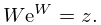
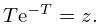
… ► $\ln z$ is a single-valued analytic function on $ℂ\setminus (-\mathrm{\infty },0]$ and real-valued when $z$ ranges over the positive real numbers. … ►Most texts extend the definition of the principal value to include the branch cut … ►As a consequence, it has the advantage of extending regions of validity of properties of principal values. … ►The function $\exp$ is an entire function of $z$, with no real or complex zeros. … ►This is an analytic function of $z$ on $ℂ\setminus (-\mathrm{\infty },0]$, and is two-valued and discontinuous on the cut shown in Figure 4.2.1, unless $a\in \mathbb{Z}$. …

14: 18.2 General Orthogonal Polynomials

… ►It is assumed throughout this chapter that for each polynomial $p_n(x)$ that is orthogonal on an open interval $(a,b)$ the variable $x$ is confined to the closure of $(a,b)$ unless indicated otherwise. (However, under appropriate conditions almost all equations given in the chapter can be continued analytically to various complex values of the variables.) … ►

18.2.33 $$p_{n-1}^{(1)}(z)=\frac{1}{{\mu }_0}{\int }_a^b\frac{p_n(z)-p_n(x)}{z-x}d\mu (x),$$ $z\in ℂ\backslash [a,b]$, $n=1,2,\mathrm{\dots }$,

ⓘ

Symbols:

$[a,b]$: closed interval, $ℂ$: complex plane, $dx$: differential of $x$ , $\in$: element of, $\int$: integral, $p_n(x)$: polynomial of degree $n$ , $z$: complex variable, $n$: nonnegative integer and $x$: real variable

Proved:

Chihara (1978, Chapter III, §4)(proved)

Permalink:

http://dlmf.nist.gov/18.2.E33

Encodings:

pMML, png, TeX

See also:

Annotations for §18.2(x), §18.2 and Ch.18

… ►

18.2.38 $$\underset{n\to \mathrm{\infty }}{lim}{F}_n(z)=\frac{1}{{\mu }_0}{\int }_a^b\frac{d\mu (x)}{z-x},$$ $z\in ℂ\backslash [a,b]$.

ⓘ

Symbols:

$[a,b]$: closed interval, $ℂ$: complex plane, $dx$: differential of $x$ , $\in$: element of, $\int$: integral, $z$: complex variable, $n$: nonnegative integer and $x$: real variable

Proved:

Chihara (1978, Chapter III, Theorem 4.3)(proved)

Referenced by:

§18.40(ii)

Permalink:

http://dlmf.nist.gov/18.2.E38

Encodings:

pMML, png, TeX

See also:

Annotations for §18.2(x), §18.2 and Ch.18

… ►See also the extended development of these ideas in §§18.30(vi), 18.30(vii), and in §18.40(ii) where they form the basis for one method of solving the classical moment problem. … ►For OP’s $p_n(x)$ with weight function in the class $𝒢$ there are asymptotic formulas as $n\to \mathrm{\infty }$, respectively for $x\in ℂ$ outside $[-1,1]$ and for $x\in [-1,1]$, see Szegő (1975, Theorems 12.1.2, 12.1.4). …

15: 4.23 Inverse Trigonometric Functions

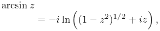
… ►The principal values (or principal branches) of the inverse sine, cosine, and tangent are obtained by introducing cuts in the $z$-plane as indicated in Figures 4.23.1(i) and 4.23.1(ii), and requiring the integration paths in (4.23.1)–(4.23.3) not to cross these cuts. … ►These functions are analytic in the cut plane depicted in Figures 4.23.1(iii) and 4.23.1(iv). … ►

…

Figure 4.23.1: $z$-plane. …

… ►This section also includes conformal mappings, and surface plots for complex arguments. … ►

4.23.19 $$\arcsin z=-\mathrm{i}\ln \left({(1-z^2)}^{1/2}+\mathrm{i}z\right),$$ $z\in ℂ\setminus (-\mathrm{\infty },-1)\cup (1,\mathrm{\infty })$;

ⓘ

Symbols:

$ℂ$: complex plane, $\in$: element of, $\mathrm{i}$: imaginary unit, $\arcsin z$: arcsine function, $\ln z$: principal branch of logarithm function, $(a,b)$: open interval, $\setminus$: set subtraction, $\cup$: union and $z$: complex variable

Referenced by:

§4.23(iv)

Permalink:

http://dlmf.nist.gov/4.23.E19

Encodings:

pMML, png, TeX

See also:

Annotations for §4.23(iv), §4.23(iv), §4.23 and Ch.4

…

16: 1.18 Linear Second Order Differential Operators and Eigenfunction Expansions

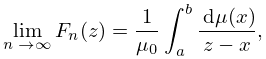
… ►If ${sup}_{v\in 𝒟(T),\Vert v\Vert =1}\Vert Tv\Vert$ is finite then $T$ is bounded, and $T$ extends uniquely to a bounded linear operator on $V$. … ►For generalizations see the Weber transform (10.22.78) and an extended Bessel transform (10.22.79). … ►Note that the integral in (1.18.66) is not singular if approached separately from above, or below, the real axis: in fact analytic continuation from the upper half of the complex plane, across the cut, and onto higher Riemann Sheets can access complex poles with singularities at discrete energies ${\lambda }_{\mathrm{res}}-\mathrm{i}{\mathrm{\Gamma }}_{\mathrm{res}}/2$ corresponding to quantum resonances, or decaying quantum states with lifetimes proportional to $1/{\mathrm{\Gamma }}_{\mathrm{res}}$. … ►The spectrum $𝝈(T)$ is the complement in $ℂ$ of $\rho (T)$. …If $T$ is a bounded operator then its spectrum is a closed bounded subset of $ℂ$. …

17: 7.12 Asymptotic Expansions

… ►

7.12.2 $$\mathrm{f}\left(z\right)\sim \frac{1}{\pi z}\sum _{m=0}^{\mathrm{\infty }}{(-1)}^m\frac{{\left(\frac{1}{2}\right)}_{2m}}{{(\pi z^2/2)}^{2m}},$$

ⓘ

Symbols:

$\mathrm{f}\left(z\right)$: auxiliary function for Fresnel integrals, ${\left(a\right)}_n$: Pochhammer’s symbol (or shifted factorial), $\sim$: Poincaré asymptotic expansion, $\pi$: the ratio of the circumference of a circle to its diameter and $z$: complex variable

A&S Ref:

7.3.27

Referenced by:

§7.12(ii), §7.12(ii), Erratum (V1.0.9) for Chapters 7, 25

Permalink:

http://dlmf.nist.gov/7.12.E2

Encodings:

pMML, png, TeX

Notational Change (effective with 1.0.9):

Previously the RHS of this equation was written as $\frac{1}{\pi z}{\sum }_{m=0}^{\mathrm{\infty }}{(-1)}^m\frac{1\cdot 3\cdot 5\mathrm{\cdots }(4m-1)}{{(\pi z^2)}^{2m}}$. We have rewritten the sum more concisely using Pochhammer’s symbol.

Suggested 2014-03-13 by Giorgos Karagounis

See also:

Annotations for §7.12(ii), §7.12 and Ch.7

►

7.12.3 $$\mathrm{g}\left(z\right)\sim \frac{1}{\pi z}\sum _{m=0}^{\mathrm{\infty }}{(-1)}^m\frac{{\left(\frac{1}{2}\right)}_{2m+1}}{{(\pi z^2/2)}^{2m+1}},$$

ⓘ

Symbols:

$\mathrm{g}\left(z\right)$: auxiliary function for Fresnel integrals, ${\left(a\right)}_n$: Pochhammer’s symbol (or shifted factorial), $\sim$: Poincaré asymptotic expansion, $\pi$: the ratio of the circumference of a circle to its diameter and $z$: complex variable

A&S Ref:

7.3.28

Referenced by:

§7.12(ii), §7.12(ii), Erratum (V1.0.9) for Chapters 7, 25

Permalink:

http://dlmf.nist.gov/7.12.E3

Encodings:

pMML, png, TeX

Notational Change (effective with 1.0.9):

Previously the RHS of this equation was written as $\frac{1}{{\pi }^2{z}^3}{\sum }_{m=0}^{\mathrm{\infty }}{(-1)}^m\frac{1\cdot 3\cdot 5\mathrm{\cdots }(4m+1)}{{(\pi z^2)}^{2m}}$ We have rewritten the sum more concisely using Pochhammer’s symbol.

Suggested 2014-03-13 by Giorgos Karagounis

See also:

Annotations for §7.12(ii), §7.12 and Ch.7

… ►

7.12.6 $$R_n^{(\mathrm{f})}(z)=\frac{{(-1)}^n}{\pi \sqrt{2}}{\int }_0^{\mathrm{\infty }}\frac{{\mathrm{e}}^{-\pi z^{2}t/2}{t}^{2n-(1/2)}}{t^2+1}dt,$$

ⓘ

Defines:

$R_n^{(\mathrm{f})}(z)$: remainder term (locally)

Symbols:

$\pi$: the ratio of the circumference of a circle to its diameter, $dx$: differential of $x$ , $\mathrm{e}$: base of natural logarithm, $\int$: integral, $z$: complex variable and $n$: nonnegative integer

A&S Ref:

7.3.29 (in different form)

Referenced by:

§7.12(ii)

Permalink:

http://dlmf.nist.gov/7.12.E6

Encodings:

pMML, png, TeX

See also:

Annotations for §7.12(ii), §7.12 and Ch.7

►

7.12.7 $$R_n^{(\mathrm{g})}(z)=\frac{{(-1)}^n}{\pi \sqrt{2}}{\int }_0^{\mathrm{\infty }}\frac{{\mathrm{e}}^{-\pi z^{2}t/2}{t}^{2n+(1/2)}}{t^2+1}dt.$$

ⓘ

Defines:

$R_n^{(\mathrm{g})}(z)$: remainder term (locally)

Symbols:

$\pi$: the ratio of the circumference of a circle to its diameter, $dx$: differential of $x$ , $\mathrm{e}$: base of natural logarithm, $\int$: integral, $z$: complex variable and $n$: nonnegative integer

A&S Ref:

7.3.30 (in different form)

Referenced by:

§7.12(ii)

Permalink:

http://dlmf.nist.gov/7.12.E7

Encodings:

pMML, png, TeX

See also:

Annotations for §7.12(ii), §7.12 and Ch.7

… ►See Olver (1997b, p. 115) for an expansion of $G\left(z\right)$ with bounds for the remainder for real and complex values of $z$.

18: 3.11 Approximation Techniques

… ►

Complex Variables

►If $x$ is replaced by a complex variable $z$ and $f(z)$ is analytic, then the expansion (3.11.11) converges within an ellipse. However, in general (3.11.11) affords no advantage in $ℂ$ for numerical purposes compared with the Maclaurin expansion of $f(z)$. ►For further details on Chebyshev-series expansions in the complex plane, see Mason and Handscomb (2003, §5.10). … ►The theory of polynomial minimax approximation given in §3.11(i) can be extended to the case when $p_n(x)$ is replaced by a rational function $R_{k,\mathrm{\ell }}(x)$. …

19: 4.13 Lambert $W$-Function

… ►

4.13.1 $$W{\mathrm{e}}^W=z.$$

ⓘ

Defines:

$W\left(z\right)$: Lambert $W$-function

Symbols:

$\mathrm{e}$: base of natural logarithm and $z$: complex variable

Referenced by:

§4.13

Permalink:

http://dlmf.nist.gov/4.13.E1

Encodings:

pMML, png, TeX

See also:

Annotations for §4.13 and Ch.4

… ► $W_0\left(z\right)$ is a single-valued analytic function on $ℂ\setminus (-\mathrm{\infty },-{\mathrm{e}}^{-1}]$, real-valued when $z>-{\mathrm{e}}^{-1}$, and has a square root branch point at $z=-{\mathrm{e}}^{-1}$. …The other branches $W_k\left(z\right)$ are single-valued analytic functions on $ℂ\setminus (-\mathrm{\infty },0]$, have a logarithmic branch point at $z=0$, and, in the case $k=\pm 1$, have a square root branch point at $z=-{\mathrm{e}}^{-1}\mp 0\mathrm{i}$ respectively. … ►

4.13.1_3 $$T{\mathrm{e}}^{-T}=z.$$

ⓘ

Symbols:

$T\left(z\right)$: Tree $T$-function, $\mathrm{e}$: base of natural logarithm and $z$: complex variable

Referenced by:

§4.13, Erratum (V1.1.7) for Expansion

Permalink:

http://dlmf.nist.gov/4.13.E1_3

Encodings:

pMML, png, TeX

Addition (effective with 1.1.7):

This equation was added.

See also:

Annotations for §4.13 and Ch.4

… ►

4.13.5_1 $${\left(\frac{W_0\left(z\right)}{z}\right)}^a={\mathrm{e}}^{-a{W}_0\left(z\right)}=\sum _{n=0}^{\mathrm{\infty }}\frac{a{\left(n+a\right)}^{n-1}}{n!}{\left(-z\right)}^n,$$ , $a\in ℂ$.

ⓘ

Symbols:

$W\left(z\right)$: Lambert $W$-function, $ℂ$: complex plane, $\in$: element of, $\mathrm{e}$: base of natural logarithm, $!$: factorial (as in $n!$), $n$: integer, $a$: real or complex constant and $z$: complex variable

Notes:

See Corless et al. (1996, formula (2.36)).

Referenced by:

§4.13, Erratum (V1.1.7) for Expansion

Permalink:

http://dlmf.nist.gov/4.13.E5_1

Encodings:

pMML, png, TeX

Addition (effective with 1.1.7):

This equation was added.

See also:

Annotations for §4.13 and Ch.4

…

20: 1.10 Functions of a Complex Variable

… ►Let $C$ be a simple closed contour consisting of a segment $\mathrm{𝐴𝐵}$ of the real axis and a contour in the upper half-plane joining the ends of $\mathrm{𝐴𝐵}$. … ►(a) By introducing appropriate cuts from the branch points and restricting $F(z)$ to be single-valued in the cut plane (or domain). … ►Branches of $F(z)$ can be defined, for example, in the cut plane $D$ obtained from $ℂ$ by removing the real axis from $1$ to $\mathrm{\infty }$ and from $-1$ to $-\mathrm{\infty }$; see Figure 1.10.1. … ►

Extended Inversion Theorem

… ► …