.%E6%96%B0%E5%AE%9D2%E4%B8%96%E7%95%8C%E6%9D%AF%E7%BB%93%E6%9D%9F%E3%80%8E%E4%B8%96%E7%95%8C%E6%9D%AF%E4%BD%A3%E9%87%91%E5%88%86%E7%BA%A255%25%EF%BC%8C%E5%92%A8%E8%AF%A2%E4%B8%93%E5%91%98%EF%BC%9A%40ky975%E3%80%8F.tbx-k2q1w9-2022%E5%B9%B411%E6%9C%8829%E6%97%A54%E6%97%B659%E5%88%8617%E7%A7%92

SearchAdvancedHelp

Did you mean .%E6%96%B0%E5%AE%9D2%E4%B8%96%E7%95%8C%E6%9D%AF%E7%BB%93%E6%9D%9F%E3%80%8E%E4%B8%96%E7%95%8C%E6%9D%AF%E4%BD%A3%E9%87%91%E5%88%86%E7%BA%255%25%EF%BC%8C%E5%92%A8%E8%AF%A2%E4%B8%93%E5%91%98%EF%BC%9A%40ky975%E3%80%8F.tbx-k2q1w9-2022%E5%B9%411%E6%9C%882%E6%97%254%E6%97%659%E5%88%86178%E7%A7%92 ?

(0.038 seconds)

1—10 of 626 matching pages

1: 34.6 Definition: $\mathit{9}j$ Symbol

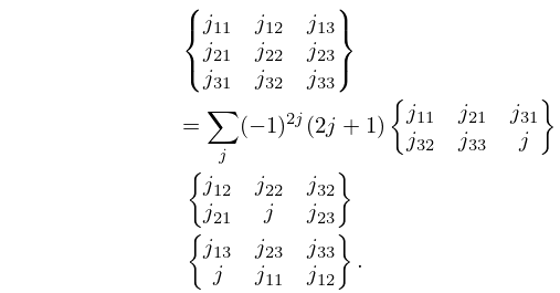
§34.6 Definition: $\mathit{9}j$ Symbol

►The $\mathit{9}j$ symbol may be defined either in terms of $\mathit{3}j$ symbols or equivalently in terms of $\mathit{6}j$ symbols: ►

34.6.1

ⓘ

Defines:

: $\mathit{9}j$ symbol

Symbols:

: $\mathit{3}j$ symbol, $j,j_r$: non-negative integers or non-negative integers plus one half., $r$: nonnegative integer and $s$: integer

Permalink:

http://dlmf.nist.gov/34.6.E1

Encodings:

pMML, png, TeX

See also:

Annotations for §34.6 and Ch.34

►

34.6.2

ⓘ

Symbols:

: $\mathit{9}j$ symbol, : $\mathit{6}j$ symbol and $j,j_r$: non-negative integers or non-negative integers plus one half.

Referenced by:

§34.13

Permalink:

http://dlmf.nist.gov/34.6.E2

Encodings:

pMML, png, TeX

See also:

Annotations for §34.6 and Ch.34

►The $\mathit{9}j$ symbol may also be written as a finite triple sum equivalent to a terminating generalized hypergeometric series of three variables with unit arguments. …

2: 26.5 Lattice Paths: Catalan Numbers

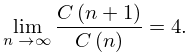
… ► $C\left(n\right)$ is the Catalan number. …(Sixty-six equivalent definitions of $C\left(n\right)$ are given in Stanley (1999, pp. 219–229).) … ►

26.5.3 $$C\left(n+1\right)=\sum _{k=0}^{n}C\left(k\right)C\left(n-k\right),$$

ⓘ

Symbols:

$C\left(n\right)$: Catalan number, $k$: nonnegative integer and $n$: nonnegative integer

Permalink:

http://dlmf.nist.gov/26.5.E3

Encodings:

pMML, png, TeX

See also:

Annotations for §26.5(iii), §26.5 and Ch.26

►

26.5.4 $$C\left(n+1\right)=\frac{2(2n+1)}{n+2}C\left(n\right),$$

ⓘ

Symbols:

$C\left(n\right)$: Catalan number and $n$: nonnegative integer

Permalink:

http://dlmf.nist.gov/26.5.E4

Encodings:

pMML, png, TeX

See also:

Annotations for §26.5(iii), §26.5 and Ch.26

… ►

26.5.7 $$\underset{n\to \mathrm{\infty }}{lim}\frac{C\left(n+1\right)}{C\left(n\right)}=4.$$

ⓘ

Symbols:

$C\left(n\right)$: Catalan number and $n$: nonnegative integer

Permalink:

http://dlmf.nist.gov/26.5.E7

Encodings:

pMML, png, TeX

See also:

Annotations for §26.5(iv), §26.5 and Ch.26

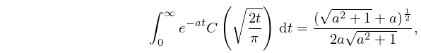
3: 6.14 Integrals

… ►

6.14.1 $${\int }_0^{\mathrm{\infty }}{\mathrm{e}}^{-at}{E}_1\left(t\right)dt=\frac{1}{a}\ln \left(1+a\right),$$ $\mathrm{\Re }a>-1$,

ⓘ

Symbols:

$dx$: differential of $x$ , $\mathrm{e}$: base of natural logarithm, $E_1\left(z\right)$: exponential integral, $\int$: integral, $\ln z$: principal branch of logarithm function and $\mathrm{\Re }$: real part

A&S Ref:

5.1.34 (special case of)

Permalink:

http://dlmf.nist.gov/6.14.E1

Encodings:

pMML, png, TeX

See also:

Annotations for §6.14(i), §6.14 and Ch.6

… ►

6.14.4 $${\int }_0^{\mathrm{\infty }}{E}_1^2\left(t\right)dt=2\ln 2,$$

ⓘ

Symbols:

$dx$: differential of $x$ , $E_1\left(z\right)$: exponential integral, $\int$: integral and $\ln z$: principal branch of logarithm function

A&S Ref:

5.1.33

Permalink:

http://dlmf.nist.gov/6.14.E4

Encodings:

pMML, png, TeX

See also:

Annotations for §6.14(ii), §6.14 and Ch.6

… ►For collections of integrals, see Apelblat (1983, pp. 110–123), Bierens de Haan (1939, pp. 373–374, 409, 479, 571–572, 637, 664–673, 680–682, 685–697), Erdélyi et al. (1954a, vol. 1, pp. 40–42, 96–98, 177–178, 325), Geller and Ng (1969), Gradshteyn and Ryzhik (2000, §§5.2–5.3 and 6.2–6.27), Marichev (1983, pp. 182–184), Nielsen (1906b), Oberhettinger (1974, pp. 139–141), Oberhettinger (1990, pp. 53–55 and 158–160), Oberhettinger and Badii (1973, pp. 172–179), Prudnikov et al. (1986b, vol. 2, pp. 24–29 and 64–92), Prudnikov et al. (1992a, §§3.4–3.6), Prudnikov et al. (1992b, §§3.4–3.6), and Watrasiewicz (1967).

4: 5.13 Integrals

…

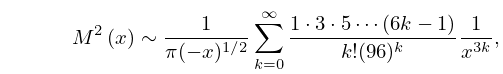
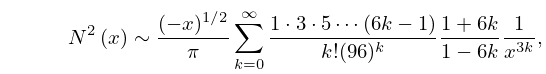
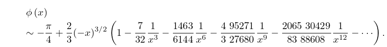
5: 9.8 Modulus and Phase

… ►

9.8.20 $$M^2\left(x\right)\sim \frac{1}{\pi {(-x)}^{1/2}}\sum _{k=0}^{\mathrm{\infty }}\frac{1\cdot 3\cdot 5\mathrm{\cdots }(6k-1)}{k!{(96)}^k}\frac{1}{x^{3k}},$$

ⓘ

Symbols:

$\sim$: Poincaré asymptotic expansion, $\pi$: the ratio of the circumference of a circle to its diameter, $!$: factorial (as in $n!$), $M\left(z\right)$: Airy modulus function and $x$: real variable

Proof sketch:

Combine (9.8.9)–(9.8.12) with §10.18(iii)

Referenced by:

§9.8(iv)

Permalink:

http://dlmf.nist.gov/9.8.E20

Encodings:

pMML, png, TeX

See also:

Annotations for §9.8(iv), §9.8 and Ch.9

►

9.8.21 $$N^2\left(x\right)\sim \frac{{(-x)}^{1/2}}{\pi }\sum _{k=0}^{\mathrm{\infty }}\frac{1\cdot 3\cdot 5\mathrm{\cdots }(6k-1)}{k!{(96)}^k}\frac{1+6k}{1-6k}\frac{1}{x^{3k}},$$

ⓘ

Symbols:

$\sim$: Poincaré asymptotic expansion, $\pi$: the ratio of the circumference of a circle to its diameter, $!$: factorial (as in $n!$), $N\left(z\right)$: Airy modulus function and $x$: real variable

Proof sketch:

Combine (9.8.9)–(9.8.12) with §10.18(iii)

Referenced by:

§9.8(iv)

Permalink:

http://dlmf.nist.gov/9.8.E21

Encodings:

pMML, png, TeX

See also:

Annotations for §9.8(iv), §9.8 and Ch.9

►

9.8.22 $$\theta \left(x\right)\sim \frac{\pi }{4}+\frac{2}{3}{(-x)}^{3/2}\left(1+\frac{5}{32}\frac{1}{x^3}+\frac{1105}{6144}\frac{1}{x^6}+\frac{82825}{65536}\frac{1}{x^9}+\frac{\mathrm{12820\hspace{0.33em}31525}}{\mathrm{587\hspace{0.33em}20256}}\frac{1}{x^{12}}+\mathrm{\cdots }\right),$$

ⓘ

Symbols:

$\sim$: Poincaré asymptotic expansion, $\pi$: the ratio of the circumference of a circle to its diameter, $\theta \left(z\right)$: Airy phase function and $x$: real variable

Proof sketch:

Combine (9.8.9)–(9.8.12) with §10.18(iii). See also Nemes (2021, Theorem 2.1 and p. 4333).

Referenced by:

§9.8(iv), §9.8(iv), Erratum (V1.1.8) for Section 9.8(iv)

Permalink:

http://dlmf.nist.gov/9.8.E22

Encodings:

pMML, png, TeX

See also:

Annotations for §9.8(iv), §9.8 and Ch.9

►

9.8.23 $$\varphi \left(x\right)\sim -\frac{\pi }{4}+\frac{2}{3}{(-x)}^{3/2}\left(1-\frac{7}{32}\frac{1}{x^3}-\frac{1463}{6144}\frac{1}{x^6}-\frac{\mathrm{4\hspace{0.33em}95271}}{\mathrm{3\hspace{0.33em}27680}}\frac{1}{x^9}-\frac{\mathrm{2065\hspace{0.33em}30429}}{\mathrm{83\hspace{0.33em}88608}}\frac{1}{x^{12}}-\mathrm{\cdots }\right).$$

ⓘ

Symbols:

$\sim$: Poincaré asymptotic expansion, $\pi$: the ratio of the circumference of a circle to its diameter, $\varphi \left(z\right)$: Airy phase function and $x$: real variable

Proof sketch:

Combine (9.8.9)–(9.8.12) with §10.18(iii). See also Nemes (2021, Theorem 2.1 and p. 4333).

Referenced by:

§9.8(iv), §9.8(iv), §9.8(iv), Erratum (V1.1.8) for Section 9.8(iv)

Permalink:

http://dlmf.nist.gov/9.8.E23

Encodings:

pMML, png, TeX

See also:

Annotations for §9.8(iv), §9.8 and Ch.9

… ►Also, approximate values (25S) of the coefficients of the powers $x^{-15}$, $x^{-18}$, $\mathrm{\dots }$, $x^{-56}$ are available in Sherry (1959). …

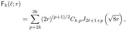
6: 33.20 Expansions for Small $|ϵ|$

… ►where ►

33.20.4 $${𝖥}_k(\mathrm{\ell };r)=\sum _{p=2k}^{3k}{(2r)}^{(p+1)/2}{C}_{k,p}{J}_{2\mathrm{\ell }+1+p}\left(\sqrt{8r}\right),$$ $r>0$,

ⓘ

Symbols:

$J_{\nu }\left(z\right)$: Bessel function of the first kind, $k$: nonnegative integer, $\mathrm{\ell }$: nonnegative integer, $r$: real variable, ${𝖥}_k(\mathrm{\ell };r)$: coefficient and $C_{k,p}$: coefficients

Permalink:

http://dlmf.nist.gov/33.20.E4

Encodings:

pMML, png, TeX

See also:

Annotations for §33.20(ii), §33.20 and Ch.33

… ►The functions $J$ and $I$ are as in §§10.2(ii), 10.25(ii), and the coefficients $C_{k,p}$ are given by $C_{0,0}=1$, $C_{1,0}=0$, and … ►where $A(ϵ,\mathrm{\ell })$ is given by (33.14.11), (33.14.12), and …The functions $Y$ and $K$ are as in §§10.2(ii), 10.25(ii), and the coefficients $C_{k,p}$ are given by (33.20.6). …

7: 7.14 Integrals

… ►

7.14.1 $${\int }_0^{\mathrm{\infty }}{\mathrm{e}}^{2\mathrm{i}at}\mathrm{erfc}\left(bt\right)dt=\frac{1}{a\sqrt{\pi }}F\left(\frac{a}{b}\right)+\frac{\mathrm{i}}{2a}\left(1-{\mathrm{e}}^{-{(a/b)}^2}\right),$$ $a\in ℂ$, .

ⓘ

Symbols:

$F\left(z\right)$: Dawson’s integral, $\pi$: the ratio of the circumference of a circle to its diameter, $\mathrm{erfc}z$: complementary error function, $ℂ$: complex plane, $dx$: differential of $x$ , $\in$: element of, $\mathrm{e}$: base of natural logarithm, $\mathrm{i}$: imaginary unit, $\int$: integral and $\mathrm{ph}$: phase

A&S Ref:

7.4.18 (in different form)

Referenced by:

§7.14(i)

Permalink:

http://dlmf.nist.gov/7.14.E1

Encodings:

pMML, png, TeX

See also:

Annotations for §7.14(i), §7.14(i), §7.14 and Ch.7

… ►

7.14.5 $${\int }_0^{\mathrm{\infty }}{\mathrm{e}}^{-at}C\left(t\right)dt=\frac{1}{a}\mathrm{f}\left(\frac{a}{\pi }\right),$$ $\mathrm{\Re }a>0$,

ⓘ

Symbols:

$\mathrm{f}\left(z\right)$: auxiliary function for Fresnel integrals, $C\left(z\right)$: Fresnel integral, $\pi$: the ratio of the circumference of a circle to its diameter, $dx$: differential of $x$ , $\mathrm{e}$: base of natural logarithm, $\int$: integral and $\mathrm{\Re }$: real part

Keywords:

Laplace transform

A&S Ref:

7.4.27 (in different notation)

Referenced by:

§7.14(ii)

Permalink:

http://dlmf.nist.gov/7.14.E5

Encodings:

pMML, png, TeX

See also:

Annotations for §7.14(ii), §7.14(ii), §7.14 and Ch.7

… ►

7.14.7 $${\int }_0^{\mathrm{\infty }}{\mathrm{e}}^{-at}C\left(\sqrt{\frac{2t}{\pi }}\right)dt=\frac{{(\sqrt{a^2+1}+a)}^{\frac{1}{2}}}{2a\sqrt{a^2+1}},$$ $\mathrm{\Re }a>0$,

ⓘ

Symbols:

$C\left(z\right)$: Fresnel integral, $\pi$: the ratio of the circumference of a circle to its diameter, $dx$: differential of $x$ , $\mathrm{e}$: base of natural logarithm, $\int$: integral and $\mathrm{\Re }$: real part

Keywords:

Laplace transform

A&S Ref:

7.4.29 in modified form

Referenced by:

§7.14(ii)

Permalink:

http://dlmf.nist.gov/7.14.E7

Encodings:

pMML, png, TeX

See also:

Annotations for §7.14(ii), §7.14(ii), §7.14 and Ch.7

… ►For collections of integrals see Apelblat (1983, pp. 131–146), Erdélyi et al. (1954a, vol. 1, pp. 40, 96, 176–177), Geller and Ng (1971), Gradshteyn and Ryzhik (2000, §§5.4 and 6.28–6.32), Marichev (1983, pp. 184–189), Ng and Geller (1969), Oberhettinger (1974, pp. 138–139, 142–143), Oberhettinger (1990, pp. 48–52, 155–158), Oberhettinger and Badii (1973, pp. 171–172, 179–181), Prudnikov et al. (1986b, vol. 2, pp. 30–36, 93–143), Prudnikov et al. (1992a, §§3.7–3.8), and Prudnikov et al. (1992b, §§3.7–3.8). …

8: 4.40 Integrals

… ►Extensive compendia of indefinite and definite integrals of hyperbolic functions include Apelblat (1983, pp. 96–109), Bierens de Haan (1939), Gröbner and Hofreiter (1949, pp. 139–160), Gröbner and Hofreiter (1950, pp. 160–167), Gradshteyn and Ryzhik (2000, Chapters 2–4), and Prudnikov et al. (1986a, §§1.4, 1.8, 2.4, 2.8).

9: Bibliography H

… ►

Certain integrals that contain a probability function. Bul. Akad. Štiince RSS Moldoven. 1975 (2), pp. 86–88, 95 (Russian).

ⓘ

External Links:

MathReview (C. Tanaka)

Referenced by:

§7.14(iii).

Encodings:

BibTeX

… ►

Expansions for the probability function in series of Čebyšev polynomials and Bessel functions. Bul. Akad. Štiince RSS Moldoven. 1976 (1), pp. 77–80, 96 (Russian).

ⓘ

External Links:

MathReview (V. L. Makarov)

Referenced by:

§7.14(iii).

Encodings:

BibTeX

►

Integrals that contain a probability function of complicated arguments. Bul. Akad. Štiince RSS Moldoven. 1976 (1), pp. 80–84, 96 (Russian).

ⓘ

External Links:

MathReview (V. L. Makarov)

Referenced by:

§7.14(iii).

Encodings:

BibTeX

►

Sums with cylindrical functions that reduce to the probability function and to related functions. Bul. Akad. Shtiintse RSS Moldoven. 1978 (3), pp. 80–84, 95 (Russian).

ⓘ

External Links:

MathReview (M. Lawrence Glasser)

Referenced by:

§7.14(iii).

Encodings:

BibTeX

… ►

Algorithm 56: Complete elliptic integral of the second kind. Comm. ACM 4 (4), pp. 180–181.

ⓘ

Notes:

Includes Algol program, maximum accuracy 8D. For certification see same journal 9 (1966), p. 12

External Links:

ISSN 0001-0782, Document

Referenced by:

§19.39(ii).

Encodings:

BibTeX

…

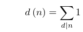
10: 27.2 Functions

… ►

27.2.9 $$d\left(n\right)=\sum _{d|n}1$$

ⓘ

Symbols:

$d_k\left(n\right)$: divisor function, $d$: positive integer and $n$: positive integer

A&S Ref:

24.3.3 I.A

Permalink:

http://dlmf.nist.gov/27.2.E9

Encodings:

pMML, png, TeX

See also:

Annotations for §27.2(i), §27.2 and Ch.27

… ►It is the special case $k=2$ of the function $d_k\left(n\right)$ that counts the number of ways of expressing $n$ as the product of $k$ factors, with the order of factors taken into account. …Note that ${\sigma }_0\left(n\right)=d\left(n\right)$. … ►Table 27.2.2 tabulates the Euler totient function $\varphi \left(n\right)$, the divisor function $d\left(n\right)$ ($={\sigma }_0(n)$), and the sum of the divisors $\sigma (n)$ ($={\sigma }_1(n)$), for $n=1(1)52$. … ►

Table 27.2.2: Functions related to division.

► ►►►

$n$	$\varphi \left(n\right)$	$d\left(n\right)$	$\sigma \left(n\right)$	$n$	$\varphi \left(n\right)$	$d\left(n\right)$	$\sigma \left(n\right)$	$n$	$\varphi \left(n\right)$	$d\left(n\right)$	$\sigma \left(n\right)$	$n$	$\varphi \left(n\right)$	$d\left(n\right)$	$\sigma \left(n\right)$
…
3	2	2	4	16	8	5	31	29	28	2	30	42	12	8	96
…

►