swallowtail catastrophe

SearchAdvancedHelp

(0.001 seconds)

10 matching pages

1: 36.2 Catastrophes and Canonical Integrals

… ►

Normal Forms Associated with Canonical Integrals: Cuspoid Catastrophe with Codimension $K$

… ►Special cases: $K=1$, fold catastrophe; $K=2$, cusp catastrophe; $K=3$, swallowtail catastrophe. …

2: 36.5 Stokes Sets

… ►

►►

Figure 36.5.2: Swallowtail catastrophe with . Magnify

►

►►

Figure 36.5.3: Swallowtail catastrophe with $z=0$. Magnify

►

►►

Figure 36.5.4: Swallowtail catastrophe with $z>0$. … Magnify

…

3: 36.4 Bifurcation Sets

… ►

►►

Figure 36.4.2: Bifurcation set of swallowtail catastrophe. Magnify

…

4: Bibliography N

… ►

Dislocation lines in the swallowtail diffraction catastrophe. Proc. Roy. Soc. Lond. Ser. A 463, pp. 343–355.

ⓘ

External Links:

ISSN 1364-5021, Document, ZentralBlatt

Referenced by:

§36.7(iv).

Encodings:

BibTeX

5: 36.6 Scaling Relations

§36.6 Scaling Relations

…

6: 36.7 Zeros

… ►The zeros of these functions are curves in $𝐱=(x,y,z)$ space; see Nye (2007) for ${\mathrm{\Phi }}_3$ and Nye (2006) for ${\mathrm{\Phi }}^{(\mathrm{H})}$.

7: Bibliography C

… ►

A differential equation method for the numerical evaluation of the Airy, Pearcey and swallowtail canonical integrals and their derivatives. Molecular Phys. 48 (6), pp. 1305–1330.

ⓘ

External Links:

ISSN 0026-8976, Document, MathReview (Peter Giblin)

Referenced by:

§36.10(i), §36.10(ii), §36.15(v), §36.8.

Encodings:

BibTeX

►

A method for the numerical evaluation of the oscillatory integrals associated with the cuspoid catastrophes: Application to Pearcey’s integral and its derivatives. J. Phys. A 15 (4), pp. 1179–1190.

ⓘ

External Links:

ISSN 0305-4470, Document, MathReview, ZentralBlatt

Referenced by:

§36.15(iii), §36.8.

Encodings:

BibTeX

►

Molecular collisions and cusp catastrophes: Three methods for the calculation of Pearcey’s integral and its derivatives. Chem. Phys. Lett. 81 (2), pp. 306–310.

ⓘ

External Links:

ISSN 0009-2614, Document, MathReview (J. S. Joel)

Referenced by:

§36.14(iii).

Encodings:

BibTeX

… ►

Catastrophes and molecular collisions. Molecular Phys. 31 (1), pp. 33–55.

ⓘ

External Links:

Document, MathReview (V. M. Zakaljukin)

Referenced by:

§36.14(iii).

Encodings:

BibTeX

…

8: 36.11 Leading-Order Asymptotics

§36.11 Leading-Order Asymptotics

… ►

36.11.2 $${\mathrm{\Psi }}_K\left(𝐱\right)=\sqrt{2\pi }\sum _{j=1}^{j_{\max }(𝐱)}\exp \left(\mathrm{i}\left({\mathrm{\Phi }}_K(t_j(𝐱);𝐱)+\frac{1}{4}\pi {(-1)}^{j+K+1}\right)\right){\left|\frac{{\partial }^2{\mathrm{\Phi }}_K(t_j(𝐱);𝐱)}{{\partial t}^2}\right|}^{-1/2}(1+o\left(1\right)).$$

ⓘ

Symbols:

${\mathrm{\Psi }}_K\left(𝐱\right)$: canonical integral function, $\pi$: the ratio of the circumference of a circle to its diameter, ${\mathrm{\Phi }}_K(t;𝐱)$: cuspoid catastrophe of codimension $K$ , $\exp z$: exponential function, $\mathrm{i}$: imaginary unit, $o\left(x\right)$: order less than, $\frac{\partial f}{\partial x}$: partial derivative of $f$ with respect to $x$ , $\partial x$: partial differential of $x$ , $t$: variable, $K$: codimension and $t_j(𝐱)$: solutions

Permalink:

http://dlmf.nist.gov/36.11.E2

Encodings:

pMML, png, TeX

See also:

Annotations for §36.11 and Ch.36

…

9: 36.10 Differential Equations

… ►

36.10.1 $${\mathrm{\Phi }}_K^{\prime }(-\mathrm{i}\frac{\partial }{\partial x_1};𝐱){\mathrm{\Psi }}_K\left(𝐱\right)=0,$$

ⓘ

Symbols:

${\mathrm{\Psi }}_K\left(𝐱\right)$: canonical integral function, ${\mathrm{\Phi }}_K(t;𝐱)$: cuspoid catastrophe of codimension $K$ , $\mathrm{i}$: imaginary unit, $\frac{\partial f}{\partial x}$: partial derivative of $f$ with respect to $x$ , $\partial x$: partial differential of $x$ , $K$: codimension and $x_{\mathrm{i}}$: real parameter

Referenced by:

§36.10(i)

Permalink:

http://dlmf.nist.gov/36.10.E1

Encodings:

pMML, png, TeX

See also:

Annotations for §36.10(i), §36.10 and Ch.36

… ► $K=3$, swallowtail: … ► $K=3$, swallowtail: … ►

►

…

10: 36.12 Uniform Approximation of Integrals

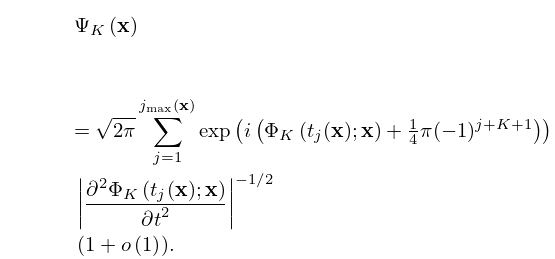
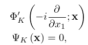
… ►Define a mapping $u(t;𝐲)$ by relating $f(u;𝐲)$ to the normal form (36.2.1) of ${\mathrm{\Phi }}_K(t;𝐱)$ in the following way: …with the $K+1$ functions $A(𝐲)$ and $𝐱(𝐲)$ determined by correspondence of the $K+1$ critical points of $f$ and ${\mathrm{\Phi }}_K$. … ►This technique can be applied to generate a hierarchy of approximations for the diffraction catastrophes ${\mathrm{\Psi }}_K(𝐱;k)$ in (36.2.10) away from $𝐱=\mathrm{𝟎}$, in terms of canonical integrals ${\mathrm{\Psi }}_J\left(\xi (𝐱;k)\right)$ for . For example, the diffraction catastrophe ${\mathrm{\Psi }}_2(x,y;k)$ defined by (36.2.10), and corresponding to the Pearcey integral (36.2.14), can be approximated by the Airy function ${\mathrm{\Psi }}_1\left(\xi (x,y;k)\right)$ when $k$ is large, provided that $x$ and $y$ are not small. … ►For further information concerning integrals with several coalescing saddle points see Arnol’d et al. (1988), Berry and Howls (1993, 1994), Bleistein (1967), Duistermaat (1974), Ludwig (1966), Olde Daalhuis (2000), and Ursell (1972, 1980).