point at infinity

SearchAdvancedHelp

(0.004 seconds)

21—30 of 77 matching pages

21: 1.4 Calculus of One Variable

… ►For the functions discussed in the following DLMF chapters these two integration measures are adequate, as these special functions are analytic functions of their variables, and thus $C^{\mathrm{\infty }}$, and well defined for all values of these variables; possible exceptions being at boundary points. …

22: 4.3 Graphics

… ►

►►

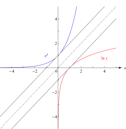
Figure 4.3.1: $\ln x$ and ${\mathrm{e}}^x$. Parallel tangent lines at $(1,0)$ and $(0,1)$ make evident the mirror symmetry across the line $y=x$, demonstrating the inverse relationship between the two functions. Magnify

… ►Corresponding points share the same letters, with bars signifying complex conjugates. Lines parallel to the real axis in the $z$-plane map onto rays in the $w$-plane, and lines parallel to the imaginary axis in the $z$-plane map onto circles centered at the origin in the $w$-plane. In the labeling of corresponding points $r$ is a real parameter that can lie anywhere in the interval $(0,\mathrm{\infty })$. …

23: 15.6 Integral Representations

… ►In (15.6.2) the point $1/z$ lies outside the integration contour, $t^{b-1}$ and ${(t-1)}^{c-b-1}$ assume their principal values where the contour cuts the interval $(1,\mathrm{\infty })$, and ${(1-zt)}^a=1$ at $t=0$. …

24: 32.11 Asymptotic Approximations for Real Variables

… ►Next, for given initial conditions $w(0)=0$ and $w^{\prime }(0)=k$, with $k$ real, $w(x)$ has at least one pole on the real axis. … ►

If , then $w(x)$ oscillates about, and is asymptotic to, $-\sqrt{\frac{1}{6}|x|}$ as $x\to -\mathrm{\infty }$.

… ►Conversely, for any nonzero real $k$, there is a unique solution $w_k(x)$ of (32.11.4) that is asymptotic to $k\mathrm{Ai}\left(x\right)$ as $x\to +\mathrm{\infty }$. … ►If $|k|>1$, then $w_k(x)$ has a pole at a finite point $x=c_0$, dependent on $k$, and … ►Now suppose $x\to -\mathrm{\infty }$. …

25: 10.25 Definitions

… ►

10.25.2 $$I_{\nu }\left(z\right)={(\frac{1}{2}z)}^{\nu }\sum _{k=0}^{\mathrm{\infty }}\frac{{(\frac{1}{4}{z}^2)}^k}{k!\mathrm{\Gamma }\left(\nu +k+1\right)}.$$

ⓘ

Defines:

$I_{\nu }\left(z\right)$: modified Bessel function of the first kind

Symbols:

$\mathrm{\Gamma }\left(z\right)$: gamma function, $!$: factorial (as in $n!$), $k$: nonnegative integer, $z$: complex variable and $\nu$: complex parameter

A&S Ref:

9.6.10

Referenced by:

§10.30(i), §10.31, §10.38, §10.45, §10.46, §10.53, §8.6(i)

Permalink:

http://dlmf.nist.gov/10.25.E2

Encodings:

pMML, png, TeX

See also:

Annotations for §10.25(ii), §10.25 and Ch.10

… ►In particular, the principal branch of $I_{\nu }\left(z\right)$ is defined in a similar way: it corresponds to the principal value of ${(\frac{1}{2}z)}^{\nu }$, is analytic in $ℂ\setminus (-\mathrm{\infty },0]$, and two-valued and discontinuous on the cut $\mathrm{ph}z=\pm \pi$. … ►as $z\to \mathrm{\infty }$ in $|\mathrm{ph}z|\le \frac{3}{2}\pi -\delta$ . It has a branch point at $z=0$ for all $\nu \in ℂ$. The principal branch corresponds to the principal value of the square root in (10.25.3), is analytic in $ℂ\setminus (-\mathrm{\infty },0]$, and two-valued and discontinuous on the cut $\mathrm{ph}z=\pm \pi$. …

26: 10.2 Definitions

… ►This differential equation has a regular singularity at $z=0$ with indices $\pm \nu$, and an irregular singularity at $z=\mathrm{\infty }$ of rank $1$; compare §§2.7(i) and 2.7(ii). … ►This solution of (10.2.1) is an analytic function of $z\in ℂ$, except for a branch point at $z=0$ when $\nu$ is not an integer. … ►Whether or not $\nu$ is an integer $Y_{\nu }\left(z\right)$ has a branch point at $z=0$. The principal branch corresponds to the principal branches of $J_{\pm \nu }\left(z\right)$ in (10.2.3) and (10.2.4), with a cut in the $z$-plane along the interval $(-\mathrm{\infty },0]$. … ►Each solution has a branch point at $z=0$ for all $\nu \in ℂ$. …

27: 15.11 Riemann’s Differential Equation

… ►The importance of (15.10.1) is that any homogeneous linear differential equation of the second order with at most three distinct singularities, all regular, in the extended plane can be transformed into (15.10.1). The most general form is given by … ►Here $\{a_1,a_2\}$, $\{b_1,b_2\}$, $\{c_1,c_2\}$ are the exponent pairs at the points $\alpha$, $\beta$, $\gamma$, respectively. …Also, if any of $\alpha$, $\beta$, $\gamma$, is at infinity, then we take the corresponding limit in (15.11.1). … ►These constants can be chosen to map any two sets of three distinct points $\{\alpha ,\beta ,\gamma \}$ and $\{\tilde{\alpha },\tilde{\beta },\tilde{\gamma }\}$ onto each other. …

28: 4.15 Graphics

… ►

►►

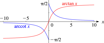
Figure 4.15.4: $\arctan x$ and $\mathrm{arccot}x$. …$\mathrm{arccot}x$ is discontinuous at $x=0$. Magnify

… ►Figure 4.15.7 illustrates the conformal mapping of the strip onto the whole $w$-plane cut along the real axis from $-\mathrm{\infty }$ to $-1$ and $1$ to $\mathrm{\infty }$, where $w=\sin z$ and $z=\arcsin w$ (principal value). Corresponding points share the same letters, with bars signifying complex conjugates. Lines parallel to the real axis in the $z$-plane map onto ellipses in the $w$-plane with foci at $w=\pm 1$, and lines parallel to the imaginary axis in the $z$-plane map onto rectangular hyperbolas confocal with the ellipses. In the labeling of corresponding points $r$ is a real parameter that can lie anywhere in the interval $(0,\mathrm{\infty })$. …

29: 2.3 Integrals of a Real Variable

… ►However, cancellation does not take place near the endpoints, owing to lack of symmetry, nor in the neighborhoods of zeros of $p^{\prime }(t)$ because $p(t)$ changes relatively slowly at these stationary points. … ►Assume that $q(t)$ again has the expansion (2.3.7) and this expansion is infinitely differentiable, $q(t)$ is infinitely differentiable on $(0,\mathrm{\infty })$, and each of the integrals $\int {\mathrm{e}}^{\mathrm{i}xt}{q}^{(s)}(t)dt$, $s=0,1,2,\mathrm{\dots }$, converges at $t=\mathrm{\infty }$, uniformly for all sufficiently large $x$. … ►For the more general integral (2.3.19) we assume, without loss of generality, that the stationary point (if any) is at the left endpoint. … ►Assume also that ${\partial }^{2}p(\alpha ,t)/{\partial t}^2$ and $q(\alpha ,t)$ are continuous in $\alpha$ and $t$, and for each $\alpha$ the minimum value of $p(\alpha ,t)$ in $[0,k)$ is at $t=\alpha$, at which point $\partial p(\alpha ,t)/\partial t$ vanishes, but both ${\partial }^{2}p(\alpha ,t)/{\partial t}^2$ and $q(\alpha ,t)$ are nonzero. When $x\to +\mathrm{\infty }$ Laplace’s method (§2.3(iii)) applies, but the form of the resulting approximation is discontinuous at $\alpha =0$. …

30: 1.18 Linear Second Order Differential Operators and Eigenfunction Expansions

… ►In unusual cases $N=\mathrm{\infty }$, even for all $\mathrm{\ell }$, such as in the case of the Schrödinger–Coulomb problem ($V=-r^{-1}$) discussed in §18.39 and §33.14, where the point spectrum actually accumulates at the onset of the continuum at $\lambda =0$, implying an essential singularity, as well as a branch point, in matrix elements of the resolvent, (1.18.66). …