in z

SearchAdvancedHelp

(0.017 seconds)

11—20 of 653 matching pages

11: 4.36 Infinite Products and Partial Fractions

… ►When $z\ne n\pi \mathrm{i}$, $n\in \mathbb{Z}$, …

12: 15.19 Methods of Computation

… ►For $z\in ℝ$ it is always possible to apply one of the linear transformations in §15.8(i) in such a way that the hypergeometric function is expressed in terms of hypergeometric functions with an argument in the interval $[0,\frac{1}{2}]$. ►For $z\in ℂ$ it is possible to use the linear transformations in such a way that the new arguments lie within the unit circle, except when $z={\mathrm{e}}^{\pm \pi \mathrm{i}/3}$. …However, by appropriate choice of the constant $z_0$ in (15.15.1) we can obtain an infinite series that converges on a disk containing $z={\mathrm{e}}^{\pm \pi \mathrm{i}/3}$. … ►The representation (15.6.1) can be used to compute the hypergeometric function in the sector . … ►For example, in the half-plane $\mathrm{\Re }z\le \frac{1}{2}$ we can use (15.12.2) or (15.12.3) to compute $F(a,b;c+N+1;z)$ and $F(a,b;c+N;z)$, where $N$ is a large positive integer, and then apply (15.5.18) in the backward direction. …

13: 7.21 Physical Applications

… ►Fried and Conte (1961) mentions the role of $w\left(z\right)$ in the theory of linearized waves or oscillations in a hot plasma; $w\left(z\right)$ is called the plasma dispersion function or Faddeeva (or Faddeyeva) function; see Faddeeva and Terent’ev (1954). …

14: 20.12 Mathematical Applications

… ►The space of complex tori $ℂ/(\mathbb{Z}+\tau \mathbb{Z})$ (that is, the set of complex numbers $z$ in which two of these numbers $z_1$ and $z_2$ are regarded as equivalent if there exist integers $m,n$ such that $z_1-z_2=m+\tau n$) is mapped into the projective space $P^3$ via the identification $z\to ({\theta }_1\left(2z\right|\tau ),{\theta }_2\left(2z\right|\tau ),{\theta }_3\left(2z\right|\tau ),{\theta }_4\left(2z\right|\tau ))$. …

15: 15.13 Zeros

… ►Let $N(a,b,c)$ denote the number of zeros of $F(a,b;c;z)$ in the sector . … ►If $a$, $b$, $c$, $c-a$, or $c-b\in \{0,-1,-2,\mathrm{\dots }\}$, then $F(a,b;c;z)$ is not defined, or reduces to a polynomial, or reduces to ${(1-z)}^{c-a-b}$ times a polynomial. …

16: 4.9 Continued Fractions

… ►valid when $z\in ℂ\setminus (-\mathrm{\infty },-1]\cup [1,\mathrm{\infty })$; see Figure 4.23.1(i). … ►For $z\in ℂ$, … ►

4.9.4 $${\mathrm{e}}^z-e_{n-1}(z)=\frac{z^n}{n!-}\frac{n!z}{(n+1)+}\frac{z}{(n+2)-}\frac{(n+1)z}{(n+3)+}\frac{2z}{(n+4)-}\frac{(n+2)z}{(n+5)+}\frac{3z}{(n+6)-}\mathrm{\cdots },$$

ⓘ

Symbols:

$\mathrm{e}$: base of natural logarithm, $!$: factorial (as in $n!$), $n$: integer, $z$: complex variable and $e_n(z)$: expansion of exponential

A&S Ref:

4.2.41

Permalink:

http://dlmf.nist.gov/4.9.E4

Encodings:

pMML, png, TeX

See also:

Annotations for §4.9(ii), §4.9 and Ch.4

… ►

4.9.5 $$e_n(z)=\sum _{k=0}^n\frac{z^k}{k!}.$$

ⓘ

Defines:

$e_n(z)$: expansion of exponential (locally)

Symbols:

$!$: factorial (as in $n!$), $k$: integer, $n$: integer and $z$: complex variable

Permalink:

http://dlmf.nist.gov/4.9.E5

Encodings:

pMML, png, TeX

See also:

Annotations for §4.9(ii), §4.9 and Ch.4

…

17: 14.21 Definitions and Basic Properties

… ► $P_{\nu }^{\pm \mu }\left(z\right)$ and ${𝑸}_{\nu }^{\mu }\left(z\right)$ exist for all values of $\nu$, $\mu$, and $z$, except possibly $z=\pm 1$ and $\mathrm{\infty }$, which are branch points (or poles) of the functions, in general. When $z$ is complex $P_{\nu }^{\pm \mu }\left(z\right)$, $Q_{\nu }^{\mu }\left(z\right)$, and ${𝑸}_{\nu }^{\mu }\left(z\right)$ are defined by (14.3.6)–(14.3.10) with $x$ replaced by $z$: the principal branches are obtained by taking the principal values of all the multivalued functions appearing in these representations when $z\in (1,\mathrm{\infty })$, and by continuity elsewhere in the $z$-plane with a cut along the interval $(-\mathrm{\infty },1]$; compare §4.2(i). The principal branches of $P_{\nu }^{\pm \mu }\left(z\right)$ and ${𝑸}_{\nu }^{\mu }\left(z\right)$ are real when $\nu$, $\mu \in ℝ$ and $z\in (1,\mathrm{\infty })$. … ►When $\mathrm{\Re }\nu \ge -\frac{1}{2}$ and $\mathrm{\Re }\mu \ge 0$, a numerically satisfactory pair of solutions of (14.21.1) in the half-plane $|\mathrm{ph}z|\le \frac{1}{2}\pi$ is given by $P_{\nu }^{-\mu }\left(z\right)$ and ${𝑸}_{\nu }^{\mu }\left(z\right)$. … ►Many of the properties stated in preceding sections extend immediately from the $x$-interval $(1,\mathrm{\infty })$ to the cut $z$-plane $ℂ\backslash (-\mathrm{\infty },1]$. …

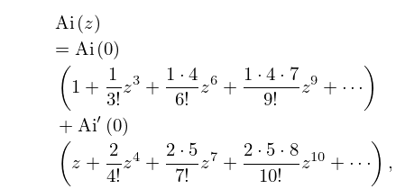
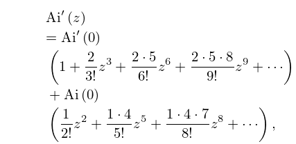
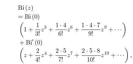
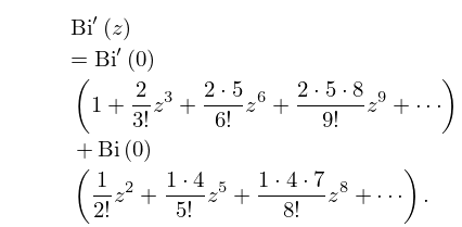
18: 9.4 Maclaurin Series

… ►For $z\in ℂ$ ►

9.4.1 $$\mathrm{Ai}\left(z\right)=\mathrm{Ai}\left(0\right)\left(1+\frac{1}{3!}{z}^3+\frac{1\cdot 4}{6!}{z}^6+\frac{1\cdot 4\cdot 7}{9!}{z}^9+\mathrm{\cdots }\right)+{\mathrm{Ai}}^{\prime }\left(0\right)\left(z+\frac{2}{4!}{z}^4+\frac{2\cdot 5}{7!}{z}^7+\frac{2\cdot 5\cdot 8}{10!}{z}^{10}+\mathrm{\cdots }\right),$$

ⓘ

Symbols:

$\mathrm{Ai}\left(z\right)$: Airy function, $!$: factorial (as in $n!$) and $z$: complex variable

Source:

Olver (1997b, p. 54)

A&S Ref:

10.4.2 (with 10.4.4 and 10.4.5)

Permalink:

http://dlmf.nist.gov/9.4.E1

Encodings:

pMML, png, TeX

See also:

Annotations for §9.4 and Ch.9

►

9.4.2 $${\mathrm{Ai}}^{\prime }\left(z\right)={\mathrm{Ai}}^{\prime }\left(0\right)\left(1+\frac{2}{3!}{z}^3+\frac{2\cdot 5}{6!}{z}^6+\frac{2\cdot 5\cdot 8}{9!}{z}^9+\mathrm{\cdots }\right)+\mathrm{Ai}\left(0\right)\left(\frac{1}{2!}{z}^2+\frac{1\cdot 4}{5!}{z}^5+\frac{1\cdot 4\cdot 7}{8!}{z}^8+\mathrm{\cdots }\right),$$

ⓘ

Symbols:

$\mathrm{Ai}\left(z\right)$: Airy function, $!$: factorial (as in $n!$) and $z$: complex variable

Proof sketch:

Use methods of Olver (1997b, p. 54).

Permalink:

http://dlmf.nist.gov/9.4.E2

Encodings:

pMML, png, TeX

See also:

Annotations for §9.4 and Ch.9

►

9.4.3 $$\mathrm{Bi}\left(z\right)=\mathrm{Bi}\left(0\right)\left(1+\frac{1}{3!}{z}^3+\frac{1\cdot 4}{6!}{z}^6+\frac{1\cdot 4\cdot 7}{9!}{z}^9+\mathrm{\cdots }\right)+{\mathrm{Bi}}^{\prime }\left(0\right)\left(z+\frac{2}{4!}{z}^4+\frac{2\cdot 5}{7!}{z}^7+\frac{2\cdot 5\cdot 8}{10!}{z}^{10}+\mathrm{\cdots }\right),$$

ⓘ

Symbols:

$\mathrm{Bi}\left(z\right)$: Airy function, $!$: factorial (as in $n!$) and $z$: complex variable

Proof sketch:

Use methods of Olver (1997b, p. 54).

A&S Ref:

10.4.3 (with 10.4.4 and 10.4.5)

Referenced by:

(9.12.15)

Permalink:

http://dlmf.nist.gov/9.4.E3

Encodings:

pMML, png, TeX

See also:

Annotations for §9.4 and Ch.9

►

9.4.4 $${\mathrm{Bi}}^{\prime }\left(z\right)={\mathrm{Bi}}^{\prime }\left(0\right)\left(1+\frac{2}{3!}{z}^3+\frac{2\cdot 5}{6!}{z}^6+\frac{2\cdot 5\cdot 8}{9!}{z}^9+\mathrm{\cdots }\right)+\mathrm{Bi}\left(0\right)\left(\frac{1}{2!}{z}^2+\frac{1\cdot 4}{5!}{z}^5+\frac{1\cdot 4\cdot 7}{8!}{z}^8+\mathrm{\cdots }\right).$$

ⓘ

Symbols:

$\mathrm{Bi}\left(z\right)$: Airy function, $!$: factorial (as in $n!$) and $z$: complex variable

Proof sketch:

Use methods of Olver (1997b, p. 54).

Permalink:

http://dlmf.nist.gov/9.4.E4

Encodings:

pMML, png, TeX

See also:

Annotations for §9.4 and Ch.9

19: 10.2 Definitions

… ►This solution of (10.2.1) is an analytic function of $z\in ℂ$, except for a branch point at $z=0$ when $\nu$ is not an integer. The principal branch of $J_{\nu }\left(z\right)$ corresponds to the principal value of ${(\frac{1}{2}z)}^{\nu }$ (§4.2(iv)) and is analytic in the $z$-plane cut along the interval $(-\mathrm{\infty },0]$. ►When $\nu =n$ $(\in \mathbb{Z})$, $J_{\nu }\left(z\right)$ is entire in $z$. … ►The principal branch corresponds to the principal branches of $J_{\pm \nu }\left(z\right)$ in (10.2.3) and (10.2.4), with a cut in the $z$-plane along the interval $(-\mathrm{\infty },0]$. … ►The principal branches correspond to principal values of the square roots in (10.2.5) and (10.2.6), again with a cut in the $z$-plane along the interval $(-\mathrm{\infty },0]$. …

20: 13.7 Asymptotic Expansions for Large Argument

… ►

13.7.4 $$U(a,b,z)=z^{-a}\sum _{s=0}^{n-1}\frac{{\left(a\right)}_s{\left(a-b+1\right)}_s}{s!}{(-z)}^{-s}+{\epsilon }_n(z),$$

ⓘ

Symbols:

$U(a,b,z)$: Kummer confluent hypergeometric function, ${\left(a\right)}_n$: Pochhammer’s symbol (or shifted factorial), $!$: factorial (as in $n!$), $n$: nonnegative integer, $s$: nonnegative integer, $z$: complex variable and ${\epsilon }_n(z)$: function

Referenced by:

§13.2(i), §13.7(ii)

Permalink:

http://dlmf.nist.gov/13.7.E4

Encodings:

pMML, png, TeX

See also:

Annotations for §13.7(ii), §13.7 and Ch.13

… ►

13.7.5 $$\left|{\epsilon }_n(z)\right|,{\beta }^{-1}\left|{\epsilon }_n^{\prime }(z)\right|\le 2\alpha C_n\left|\frac{{\left(a\right)}_n{\left(a-b+1\right)}_n}{n!z^{a+n}}\right|\exp \left(\frac{2\alpha \rho C_1}{|z|}\right),$$

ⓘ

Defines:

${\epsilon }_n(z)$: function (locally)

Symbols:

${\left(a\right)}_n$: Pochhammer’s symbol (or shifted factorial), $\exp z$: exponential function, $!$: factorial (as in $n!$), $n$: nonnegative integer, $z$: complex variable, $C_n$: coefficient, $\alpha$ , $\beta$ and $\rho$

Referenced by:

§13.2(i)

Permalink:

http://dlmf.nist.gov/13.7.E5

Encodings:

pMML, png, TeX

See also:

Annotations for §13.7(ii), §13.7 and Ch.13

… ►

13.7.7 $$z\in {\text{R}}_1,z\in {\text{R}}_2\cup {\overline{\text{R}}}_2,z\in {\text{R}}_3\cup {\overline{\text{R}}}_3,$$

ⓘ

Symbols:

$\overline{z}$: complex conjugate, $\in$: element of, $\cup$: union and $z$: complex variable

Permalink:

http://dlmf.nist.gov/13.7.E7

Encodings:

pMML, png, TeX

See also:

Annotations for §13.7(ii), §13.7 and Ch.13

… ►Also, when $z\in {\text{R}}_1\cup {\text{R}}_2\cup {\overline{\text{R}}}_2$ …and when $z\in {\text{R}}_3\cup {\overline{\text{R}}}_3$ $\sigma$ is replaced by $\nu \sigma$ and ${|z|}^{-1}$ is replaced by $\nu {|z|}^{-1}$ everywhere in (13.7.9). …