fundamental unit cell

SearchAdvancedHelp

(0.002 seconds)

1—10 of 420 matching pages

1: 22.4 Periods, Poles, and Zeros

… ►

§22.4(ii) Graphical Interpretation via Glaisher’s Notation

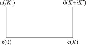
►Figure 22.4.2 depicts the fundamental unit cell in the $z$-plane, with vertices $\text{s}=0$, $\text{c}=K$, $\text{d}=K+\mathrm{i}{K}^{\prime }$, $\text{n}=\mathrm{i}{K}^{\prime }$. The set of points $z=mK+n\mathrm{i}{K}^{\prime }$, $m,n\in \mathbb{Z}$, comprise the lattice for the 12 Jacobian functions; all other lattice unit cells are generated by translation of the fundamental unit cell by $mK+n\mathrm{i}{K}^{\prime }$, where again $m,n\in \mathbb{Z}$. ►

►►

Figure 22.4.2: $z$-plane. Fundamental unit cell. Magnify

… ►Let p,q be any two distinct letters from the set s,c,d,n which appear in counterclockwise orientation at the corners of all lattice unit cells. …

2: 28.29 Definitions and Basic Properties

… ►

28.29.4 $$w_{\text{I}}(z+\pi ,\lambda )=w_{\text{I}}(\pi ,\lambda )w_{\text{I}}(z,\lambda )+w_{\text{I}}^{\prime }(\pi ,\lambda )w_{\text{II}}(z,\lambda ),$$

ⓘ

Symbols:

$\pi$: the ratio of the circumference of a circle to its diameter, $z$: complex variable, $w(z)$: Mathieu’s equation solution, $w_{\text{I}}(z;a,q)$: fundamental solution, $w_{\text{II}}(z;a,q)$: fundamental solution and $\lambda$: parameter

Permalink:

http://dlmf.nist.gov/28.29.E4

Encodings:

pMML, png, TeX

See also:

Annotations for §28.29(ii), §28.29 and Ch.28

… ►iff ${\mathrm{e}}^{\pi \mathrm{i}\nu }$ is an eigenvalue of the matrix … ►If $\nu$ $(\ne 0,1)$ is a solution of (28.29.9), then $F_{\nu }(z)$, $F_{-\nu }(z)$ comprise a fundamental pair of solutions of Hill’s equation. … ►A nontrivial solution $w(z)$ is either a Floquet solution with respect to $\nu$, or $w(z+\pi )-{\mathrm{e}}^{\mathrm{i}\nu \pi }w(z)$ is a Floquet solution with respect to $-\nu$. … ►

28.29.15 $$△(\lambda )=w_{\text{I}}(\pi ,\lambda )+w_{\text{II}}^{\prime }(\pi ,\lambda )$$

ⓘ

Symbols:

$\pi$: the ratio of the circumference of a circle to its diameter, $w_{\text{I}}(z;a,q)$: fundamental solution, $w_{\text{II}}(z;a,q)$: fundamental solution and $\lambda$: parameter

Permalink:

http://dlmf.nist.gov/28.29.E15

Encodings:

pMML, png, TeX

See also:

Annotations for §28.29(iii), §28.29 and Ch.28

…

3: 28.2 Definitions and Basic Properties

… ►(28.2.1) possesses a fundamental pair of solutions $w_{\text{I}}(z;a,q),w_{\text{II}}(z;a,q)$ called basic solutions with ►

28.2.5

ⓘ

Symbols:

$q=h^2$: parameter, $a$: parameter, $w(z)$: Mathieu’s equation solution, $w_{\text{I}}(z;a,q)$: fundamental solution and $w_{\text{II}}(z;a,q)$: fundamental solution

A&S Ref:

20.3.9 (in different notation)

Referenced by:

§28.29(ii), item (a), item (c)

Permalink:

http://dlmf.nist.gov/28.2.E5

Encodings:

pMML, png, TeX

See also:

Annotations for §28.2(ii), §28.2 and Ch.28

… ►

28.2.6 $$𝒲\left\{w_{\text{I}},w_{\text{II}}\right\}=1,$$

ⓘ

Symbols:

$𝒲$: Wronskian, $w_{\text{I}}(z;a,q)$: fundamental solution and $w_{\text{II}}(z;a,q)$: fundamental solution

Referenced by:

§28.29(ii)

Permalink:

http://dlmf.nist.gov/28.2.E6

Encodings:

pMML, png, TeX

See also:

Annotations for §28.2(ii), §28.2 and Ch.28

… ►iff ${\mathrm{e}}^{\pi \mathrm{i}\nu }$ is an eigenvalue of the matrix … ►Therefore a nontrivial solution $w(z)$ is either a Floquet solution with respect to $\nu$, or $w(z+\pi )-{\mathrm{e}}^{\mathrm{i}\nu \pi }w(z)$ is a Floquet solution with respect to $-\nu$. …

4: 16.21 Differential Equation

… ►A fundamental set of solutions of (16.21.1) is given by ►

16.21.2 $$G_{p,q}^{1,p}(z{\mathrm{e}}^{(p-m-n-1)\pi \mathrm{i}};\genfrac{}{}{0pt}{}{a_1,\mathrm{\dots },a_p}{b_j,b_1,\mathrm{\dots },b_{j-1},b_{j+1},\mathrm{\dots },b_q}),$$ $j=1,\mathrm{\dots },q$.

ⓘ

Symbols:

$G_{p,q}^{m,n}(z;\genfrac{}{}{0pt}{}{a_1,\mathrm{\dots },a_p}{b_1,\mathrm{\dots },b_q})$ or $G_{p,q}^{m,n}(z;𝐚;𝐛)$: Meijer $G$-function, $\pi$: the ratio of the circumference of a circle to its diameter, $\mathrm{e}$: base of natural logarithm, $\mathrm{i}$: imaginary unit, $p$: nonnegative integer, $q$: nonnegative integer, $z$: complex variable, $a,a_1,\mathrm{\dots },a_p$: real or complex parameters and $b,b_1,\mathrm{\dots },b_q$: real or complex parameters

Permalink:

http://dlmf.nist.gov/16.21.E2

Encodings:

pMML, png, TeX

See also:

Annotations for §16.21 and Ch.16

►For other fundamental sets see Erdélyi et al. (1953a, §5.4) and Marichev (1984).

5: 20.2 Definitions and Periodic Properties

… ►The four points $(0,\pi ,\pi +\tau \pi ,\tau \pi )$ are the vertices of the fundamental parallelogram in the $z$-plane; see Figure 20.2.1. … ►

…

Figure 20.2.1: $z$-plane. Fundamental parallelogram. …

… ►

20.2.10 $$M\equiv M(z|\tau )={\mathrm{e}}^{\mathrm{i}z+(\mathrm{i}\pi \tau /4)},$$

ⓘ

Defines:

$M$ (locally)

Symbols:

$\pi$: the ratio of the circumference of a circle to its diameter, $\equiv$: equals by definition, $\mathrm{e}$: base of natural logarithm, $\mathrm{i}$: imaginary unit, $z$: complex and $\tau$: lattice parameter

A&S Ref:

16.33.1 (in different notation)

Permalink:

http://dlmf.nist.gov/20.2.E10

Encodings:

pMML, png, TeX

See also:

Annotations for §20.2(iii), §20.2 and Ch.20

►

20.2.11 $${\theta }_1\left(z\right|\tau )=-{\theta }_2\left(z+\frac{1}{2}\pi \right|\tau )=-\mathrm{i}M{\theta }_4\left(z+\frac{1}{2}\pi \tau \right|\tau )=-\mathrm{i}M{\theta }_3\left(z+\frac{1}{2}\pi +\frac{1}{2}\pi \tau \right|\tau ),$$

ⓘ

Symbols:

${\theta }_j\left(z\right|\tau )$: theta function, $\pi$: the ratio of the circumference of a circle to its diameter, $\mathrm{i}$: imaginary unit, $z$: complex, $\tau$: lattice parameter and $M$

A&S Ref:

16.33.2 (in different notation)

Referenced by:

§20.7(iv)

Permalink:

http://dlmf.nist.gov/20.2.E11

Encodings:

pMML, png, TeX

See also:

Annotations for §20.2(iii), §20.2 and Ch.20

… ►

20.2.14 $${\theta }_4\left(z\right|\tau )={\theta }_3\left(z+\frac{1}{2}\pi \right|\tau )=-\mathrm{i}M{\theta }_1\left(z+\frac{1}{2}\pi \tau \right|\tau )=\mathrm{i}M{\theta }_2\left(z+\frac{1}{2}\pi +\frac{1}{2}\pi \tau \right|\tau ).$$

ⓘ

Symbols:

${\theta }_j\left(z\right|\tau )$: theta function, $\pi$: the ratio of the circumference of a circle to its diameter, $\mathrm{i}$: imaginary unit, $z$: complex, $\tau$: lattice parameter and $M$

Referenced by:

§20.7(iv)

Permalink:

http://dlmf.nist.gov/20.2.E14

Encodings:

pMML, png, TeX

See also:

Annotations for §20.2(iii), §20.2 and Ch.20

…

6: Howard S. Cohl

… ►Cohl has published papers in orthogonal polynomials and special functions, and is particularly interested in fundamental solutions of linear partial differential equations on Riemannian manifolds, associated Legendre functions, generalized and basic hypergeometric functions, eigenfunction expansions of fundamental solutions in separable coordinate systems for linear partial differential equations, orthogonal polynomial generating function and generalized expansions, and $q$-series. …

7: 15.10 Hypergeometric Differential Equation

… ►

§15.10(i) Fundamental Solutions

… ►When none of the exponent pairs differ by an integer, that is, when none of $c$, $c-a-b$, $a-b$ is an integer, we have the following pairs $f_1(z)$, $f_2(z)$ of fundamental solutions. … ►(a) If $c$ equals $n=1,2,3,\mathrm{\dots }$, and $a=1,2,\mathrm{\dots },n-1$, then fundamental solutions in the neighborhood of $z=0$ are given by (15.10.2) with the interpretation (15.2.5) for $f_2(z)$. … ► … ►The three pairs of fundamental solutions given by (15.10.2), (15.10.4), and (15.10.6) can be transformed into 18 other solutions by means of (15.8.1), leading to a total of 24 solutions known as Kummer’s solutions. …

8: 4.37 Inverse Hyperbolic Functions

… ►In (4.37.1) the integration path may not pass through either of the points $t=\pm \mathrm{i}$, and the function ${(1+t^2)}^{1/2}$ assumes its principal value when $t$ is real. …$\mathrm{Arcsinh}z$ and $\mathrm{Arccsch}z$ have branch points at $z=\pm \mathrm{i}$; the other four functions have branch points at $z=\pm 1$. … ►

4.37.11 $$\mathrm{arccosh}\left(-z\right)=\pm \pi \mathrm{i}+\mathrm{arccosh}z,$$ $\mathrm{\Im }z\gtrless 0$.

ⓘ

Symbols:

$\pi$: the ratio of the circumference of a circle to its diameter, $\mathrm{arccosh}z$: inverse hyperbolic cosine function, $\mathrm{\Im }$: imaginary part, $\mathrm{i}$: imaginary unit and $z$: complex variable

A&S Ref:

4.6.12 (has an error even in the tenth printing.)

Referenced by:

§4.37(iii)

Permalink:

http://dlmf.nist.gov/4.37.E11

Encodings:

pMML, png, TeX

See also:

Annotations for §4.37(iii), §4.37 and Ch.4

… ►

4.37.20 $$\mathrm{arccosh}\left(\mathrm{i}y\right)=\pm \frac{1}{2}\pi \mathrm{i}+\ln \left({(y^2+1)}^{1/2}\pm y\right),$$ $y\gtrless 0$.

ⓘ

Symbols:

$\pi$: the ratio of the circumference of a circle to its diameter, $\mathrm{arccosh}z$: inverse hyperbolic cosine function, $\mathrm{i}$: imaginary unit, $\ln z$: principal branch of logarithm function and $y$: real variable

Referenced by:

§4.37(iv)

Permalink:

http://dlmf.nist.gov/4.37.E20

Encodings:

pMML, png, TeX

See also:

Annotations for §4.37(iv), §4.37(iv), §4.37 and Ch.4

… ►

§4.37(v) Fundamental Property

…

9: 13.2 Definitions and Basic Properties

… ►

§13.2(v) Numerically Satisfactory Solutions

►Fundamental pairs of solutions of (13.2.1) that are numerically satisfactory (§2.7(iv)) in the neighborhood of infinity are … ►A fundamental pair of solutions that is numerically satisfactory near the origin is … ►When $b=n+1=1,2,3,\mathrm{\dots }$, a fundamental pair that is numerically satisfactory near the origin is $M(a,n+1,z)$ and … ► …

10: Leonard C. Maximon

… ►Maximon published numerous papers on the fundamental processes of quantum electrodynamics and on the special functions of mathematical physics. …