.put世界杯相声汇_『网址:687.vii』世界杯决赛乌龙球_b5p6v3_2022年11月30日4时58分48秒_ucgsamhsa
The terms "ucgsamhsa", "b5p6v3" were not found.Possible alternative term: "zusammenhang".
(0.004 seconds)
1—10 of 180 matching pages
1: 26.13 Permutations: Cycle Notation
…
►In cycle notation, the elements in each cycle are put inside parentheses, ordered so that immediately follows or, if is the last listed element of the cycle, then is the first element of the cycle.
…
►Again, for the example (26.13.2) a minimal decomposition into adjacent transpositions is given by : .
2: 26.17 The Twelvefold Way
…
►The twelvefold way gives the number of mappings from set of objects to set of objects (putting balls from set into boxes in set ).
…
3: Bibliography F
…
►
Algorithm 838: Airy functions.
ACM Trans. Math. Software 30 (4), pp. 491–501.
…
►
A Table of the Complete Elliptic Integral of the First Kind for Complex Values of the Modulus. Part I.
Technical report
Technical Report ARL 69-0172, Aerospace Research Laboratories, Office of Aerospace Research, Wright-Patterson Air Force Base, Ohio.
…
►
Polynomial relations in the Heisenberg algebra.
J. Math. Phys. 35 (11), pp. 6144–6149.
…
►
On a unified approach to transformations and elementary solutions of Painlevé equations.
J. Math. Phys. 23 (11), pp. 2033–2042.
…
►
Algorithm 435: Modified incomplete gamma function.
Comm. ACM 15 (11), pp. 993–995.
…
4: Guide to Searching the DLMF
…
►Be careful, however, because if you put quotes around math expressions involving math symbols, you may not get the matches you’d expect.
…
5: 19.22 Quadratic Transformations
…
►The AGM, , of two positive numbers and is defined in §19.8(i).
…where
…where and
…(If , then and (19.22.13) reduces to (19.22.11).)
…
►and the corresponding equations with , , and replaced by , , and , respectively.
…
6: 19.17 Graphics
…
►To view and for complex , put
, use (19.25.1), and see Figures 19.3.7–19.3.12.
…
►To view and for complex , put
, use (19.25.1), and see Figures 19.3.7–19.3.12.
…
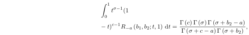
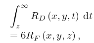
7: 19.28 Integrals of Elliptic Integrals
…
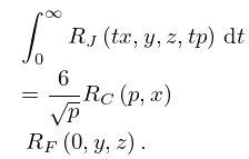
►
19.28.4
, .
…
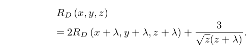
►
19.28.5
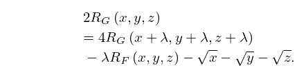
►
19.28.6
…
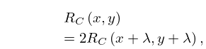
►
19.28.8
…
►To replace a single component of in by several different variables (as in (19.28.6)), see Carlson (1963, (7.9)).
…
