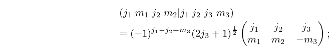
About the Project

.06世界杯阿根廷德国_『wn4.com_』世界杯球队夺冠概率_w6n2c9o_2022年11月29日15时45分40秒_w48y4c4i4

AdvancedHelp

(0.004 seconds)

11—20 of 784 matching pages

11: 34.1 Special Notation
( j 1 j 2 j 3 m 1 m 2 m 3 ) ,
{ j 1 j 2 j 3 l 1 l 2 l 3 } ,
{ j 11 j 12 j 13 j 21 j 22 j 23 j 31 j 32 j 33 } .
An often used alternative to the 3 j symbol is the Clebsch–Gordan coefficient
34.1.1 ( j 1 m 1 j 2 m 2 | j 1 j 2 j 3 m 3 ) = ( 1 ) j 1 j 2 + m 3 ( 2 j 3 + 1 ) 1 2 ( j 1 j 2 j 3 m 1 m 2 m 3 ) ;
12: 24.2 Definitions and Generating Functions
B 2 n + 1 = 0 ,
24.2.4 B n = B n ( 0 ) ,
Table 24.2.4: Euler numbers E n .
n E n
Table 24.2.5: Coefficients b n , k of the Bernoulli polynomials B n ( x ) = k = 0 n b n , k x k .
k
Table 24.2.6: Coefficients e n , k of the Euler polynomials E n ( x ) = k = 0 n e n , k x k .
k
13: 28.6 Expansions for Small q
Leading terms of the power series for a m ( q ) and b m ( q ) for m 6 are: … The coefficients of the power series of a 2 n ( q ) , b 2 n ( q ) and also a 2 n + 1 ( q ) , b 2 n + 1 ( q ) are the same until the terms in q 2 n 2 and q 2 n , respectively. … Numerical values of the radii of convergence ρ n ( j ) of the power series (28.6.1)–(28.6.14) for n = 0 , 1 , , 9 are given in Table 28.6.1. Here j = 1 for a 2 n ( q ) , j = 2 for b 2 n + 2 ( q ) , and j = 3 for a 2 n + 1 ( q ) and b 2 n + 1 ( q ) . …
§28.6(ii) Functions ce n and se n
14: 10.75 Tables
  • Achenbach (1986) tabulates J 0 ( x ) , J 1 ( x ) , Y 0 ( x ) , Y 1 ( x ) , x = 0 ( .1 ) 8 , 20D or 18–20S.

  • Makinouchi (1966) tabulates all values of j ν , m and y ν , m in the interval ( 0 , 100 ) , with at least 29S. These are for ν = 0 ( 1 ) 5 , 10, 20; ν = 3 2 , 5 2 ; ν = m / n with m = 1 ( 1 ) n 1 and n = 3 ( 1 ) 8 , except for ν = 1 2 .

  • Abramowitz and Stegun (1964, Chapter 11) tabulates 0 x J 0 ( t ) d t , 0 x Y 0 ( t ) d t , x = 0 ( .1 ) 10 , 10D; 0 x t 1 ( 1 J 0 ( t ) ) d t , x t 1 Y 0 ( t ) d t , x = 0 ( .1 ) 5 , 8D.

  • Leung and Ghaderpanah (1979), tabulates all zeros of the principal value of K n ( z ) , for n = 2 ( 1 ) 10 , 29S.

  • Abramowitz and Stegun (1964, Chapter 11) tabulates e x 0 x I 0 ( t ) d t , e x x K 0 ( t ) d t , x = 0 ( .1 ) 10 , 7D; e x 0 x t 1 ( I 0 ( t ) 1 ) d t , x e x x t 1 K 0 ( t ) d t , x = 0 ( .1 ) 5 , 6D.

  • 15: 26.12 Plane Partitions
    26.12.9 ( h = 1 r j = 1 s h + j + t 1 h + j 1 ) 2 ;
    26.12.10 ( h = 1 r j = 1 s h + j + t 1 h + j 1 ) ( h = 1 r + 1 j = 1 s h + j + t 1 h + j 1 ) ;
    26.12.11 ( h = 1 r + 1 j = 1 s h + j + t 1 h + j 1 ) ( h = 1 r j = 1 s + 1 h + j + t 1 h + j 1 ) .
    The notation π B ( r , s , t ) denotes the sum over all plane partitions contained in B ( r , s , t ) , and | π | denotes the number of elements in π . … where σ 2 ( j ) is the sum of the squares of the divisors of j . …
    16: 3.6 Linear Difference Equations
    Given numerical values of w 0 and w 1 , the solution w n of the equation …These errors have the effect of perturbing the solution by unwanted small multiples of w n and of an independent solution g n , say. … The unwanted multiples of g n now decay in comparison with w n , hence are of little consequence. … The latter method is usually superior when the true value of w 0 is zero or pathologically small. … beginning with e 0 = w 0 . …
    17: 28.35 Tables
  • Blanch and Rhodes (1955) includes 𝐵𝑒 n ( t ) , 𝐵𝑜 n ( t ) , t = 1 2 q , n = 0 ( 1 ) 15 ; 8D. The range of t is 0 to 0.1, with step sizes ranging from 0.002 down to 0.00025. Notation: 𝐵𝑒 n ( t ) = a n ( q ) + 2 q ( 4 n + 2 ) q , 𝐵𝑜 n ( t ) = b n ( q ) + 2 q ( 4 n 2 ) q .

  • Ince (1932) includes eigenvalues a n , b n , and Fourier coefficients for n = 0 or 1 ( 1 ) 6 , q = 0 ( 1 ) 10 ( 2 ) 20 ( 4 ) 40 ; 7D. Also ce n ( x , q ) , se n ( x , q ) for q = 0 ( 1 ) 10 , x = 1 ( 1 ) 90 , corresponding to the eigenvalues in the tables; 5D. Notation: a n = 𝑏𝑒 n 2 q , b n = 𝑏𝑜 n 2 q .

  • Stratton et al. (1941) includes b n , b n , and the corresponding Fourier coefficients for Se n ( c , x ) and So n ( c , x ) for n = 0 or 1 ( 1 ) 4 , c = 0 ( .1 or .2 ) 4.5 . Precision is mostly 5S. Notation: c = 2 q , b n = a n + 2 q , b n = b n + 2 q , and for Se n ( c , x ) , So n ( c , x ) see §28.1.

  • Ince (1932) includes the first zero for ce n , se n for n = 2 ( 1 ) 5 or 6 , q = 0 ( 1 ) 10 ( 2 ) 40 ; 4D. This reference also gives zeros of the first derivatives, together with expansions for small q .

  • For other tables prior to 1961 see Fletcher et al. (1962, §2.2) and Lebedev and Fedorova (1960, Chapter 11).
    18: 3.9 Acceleration of Convergence
    A transformation of a convergent sequence { s n } with limit σ into a sequence { t n } is called limit-preserving if { t n } converges to the same limit σ . … This transformation is accelerating if { s n } is a linearly convergent sequence, i. … Then the transformation of the sequence { s n } into a sequence { t n , 2 k } is given by … Then t n , 2 k = ε 2 k ( n ) . … We give a special form of Levin’s transformation in which the sequence s = { s n } of partial sums s n = j = 0 n a j is transformed into: …
    19: Bibliography
  • S. Ahmed and M. E. Muldoon (1980) On the zeros of confluent hypergeometric functions. III. Characterization by means of nonlinear equations. Lett. Nuovo Cimento (2) 29 (11), pp. 353–358.
  • D. E. Amos (1983c) Uniform asymptotic expansions for exponential integrals E n ( x ) and Bickley functions Ki n ( x ) . ACM Trans. Math. Software 9 (4), pp. 467–479.
  • K. Aomoto (1987) Special value of the hypergeometric function F 2 3 and connection formulae among asymptotic expansions. J. Indian Math. Soc. (N.S.) 51, pp. 161–221.
  • V. I. Arnol’d (1972) Normal forms of functions near degenerate critical points, the Weyl groups A k , D k , E k and Lagrangian singularities. Funkcional. Anal. i Priložen. 6 (4), pp. 3–25 (Russian).
  • V. I. Arnol’d (1974) Normal forms of functions in the neighborhood of degenerate critical points. Uspehi Mat. Nauk 29 (2(176)), pp. 11–49 (Russian).
  • 20: 3.7 Ordinary Differential Equations
    The path is partitioned at P + 1 points labeled successively z 0 , z 1 , , z P , with z 0 = a , z P = b . … Write τ j = z j + 1 z j , j = 0 , 1 , , P , expand w ( z ) and w ( z ) in Taylor series (§1.10(i)) centered at z = z j , and apply (3.7.2). … If, for example, β 0 = β 1 = 0 , then on moving the contributions of w ( z 0 ) and w ( z P ) to the right-hand side of (3.7.13) the resulting system of equations is not tridiagonal, but can readily be made tridiagonal by annihilating the elements of 𝐀 P that lie below the main diagonal and its two adjacent diagonals. … The values λ k are the eigenvalues and the corresponding solutions w k of the differential equation are the eigenfunctions. … where h = z n + 1 z n and …