.体育推单 摩登4『世界杯佣金分红55%，咨询专员：@ky975』.wua.k2q1w9-eoiyaq2o2

SearchAdvancedHelp

(0.003 seconds)

21—30 of 521 matching pages

21: Bibliography F

… ►

Algorithm 838: Airy functions. ACM Trans. Math. Software 30 (4), pp. 491–501.

ⓘ

Notes:

Single- and double-precision Fortran, maximum accuracy 32S.

External Links:

ISSN 0098-3500, Document, Code, MathReview Entry, ZentralBlatt

Referenced by:

3rd item, 2nd item, 1st item.

Encodings:

BibTeX

►

On the reversion of an asymptotic expansion and the zeros of the Airy functions. SIAM Rev. 41 (4), pp. 762–773.

ⓘ

External Links:

ISSN 1095-7200, Document, MathReview (Eberhard Wagner), ZentralBlatt

Referenced by:

§2.2, §2.2, §3.8(v), §9.9(iv), §9.9(iv).

Encodings:

BibTeX

… ►

The second Appell function for one large variable. Mediterr. J. Math. 10 (4), pp. 1853–1865.

ⓘ

External Links:

ISSN 1660-5446, Document, FullText, MathReview Entry, ZentralBlatt

Referenced by:

§16.13, §16.13.

Encodings:

BibTeX

… ►

On the reciprocal modulus relation for elliptic integrals. SIAM J. Math. Anal. 1 (4), pp. 524–526.

ⓘ

External Links:

Document, MathReview (B. C. Carlson), ZentralBlatt

Referenced by:

§19.7(i).

Encodings:

BibTeX

… ►

Numerical treatment of Coulomb wave functions. Rev. Mod. Phys. 27 (4), pp. 399–411.

ⓘ

External Links:

Document, MathReview (A. Erdélyi), ZentralBlatt

Referenced by:

§33.10(ii), §33.11, §33.12(i), §33.9(ii).

Encodings:

BibTeX

…

22: 4.17 Special Values and Limits

… ►

Table 4.17.1: Trigonometric functions: values at multiples of $\frac{1}{12}\pi$.

► ►►►►►►►

$\theta$	$\sin \theta$	$\cos \theta$	$\tan \theta$	$\csc \theta$	$\sec \theta$	$\cot \theta$
…
$\pi /12$	$\frac{1}{4}\sqrt{2}(\sqrt{3}-1)$	$\frac{1}{4}\sqrt{2}(\sqrt{3}+1)$	$2-\sqrt{3}$	$\sqrt{2}(\sqrt{3}+1)$	$\sqrt{2}(\sqrt{3}-1)$	$2+\sqrt{3}$
…
$\pi /4$	$\frac{1}{2}\sqrt{2}$	$\frac{1}{2}\sqrt{2}$	$1$	$\sqrt{2}$	$\sqrt{2}$	$1$
…
$5\pi /12$	$\frac{1}{4}\sqrt{2}(\sqrt{3}+1)$	$\frac{1}{4}\sqrt{2}(\sqrt{3}-1)$	$2+\sqrt{3}$	$\sqrt{2}(\sqrt{3}-1)$	$\sqrt{2}(\sqrt{3}+1)$	$2-\sqrt{3}$
…
$7\pi /12$	$\frac{1}{4}\sqrt{2}(\sqrt{3}+1)$	$-\frac{1}{4}\sqrt{2}(\sqrt{3}-1)$	$-(2+\sqrt{3})$	$\sqrt{2}(\sqrt{3}-1)$	$-\sqrt{2}(\sqrt{3}+1)$	$-(2-\sqrt{3})$
…
$11\pi /12$	$\frac{1}{4}\sqrt{2}(\sqrt{3}-1)$	$-\frac{1}{4}\sqrt{2}(\sqrt{3}+1)$	$-(2-\sqrt{3})$	$\sqrt{2}(\sqrt{3}+1)$	$-\sqrt{2}(\sqrt{3}-1)$	$-(2+\sqrt{3})$
…

►

…

23: 8.21 Generalized Sine and Cosine Integrals

… ►Furthermore, $\mathrm{si}(a,z)$ and $\mathrm{ci}(a,z)$ are entire functions of $a$, and $\mathrm{Si}(a,z)$ and $\mathrm{Ci}(a,z)$ are meromorphic functions of $a$ with simple poles at $a=-1,-3,-5,\mathrm{\dots }$ and $a=0,-2,-4,\mathrm{\dots }$, respectively. … ►When $\mathrm{ph}z=0$ (and when $a\ne -1,-3,-5,\mathrm{\dots }$, in the case of $\mathrm{Si}(a,z)$, or $a\ne 0,-2,-4,\mathrm{\dots }$, in the case of $\mathrm{Ci}(a,z)$) the principal values of $\mathrm{si}(a,z)$, $\mathrm{ci}(a,z)$, $\mathrm{Si}(a,z)$, and $\mathrm{Ci}(a,z)$ are defined by (8.21.1) and (8.21.2) with the incomplete gamma functions assuming their principal values (§8.2(i)). … ►

8.21.9 $$\mathrm{Ci}(a,z)=\mathrm{\Gamma }\left(a\right)\cos \left(\frac{1}{2}\pi a\right)-\mathrm{ci}(a,z),$$ $a\ne 0,-2,-4,\mathrm{\dots }$.

ⓘ

Symbols:

$\mathrm{\Gamma }\left(z\right)$: gamma function, $\pi$: the ratio of the circumference of a circle to its diameter, $\cos z$: cosine function, $\mathrm{Ci}(a,z)$: generalized cosine integral, $\mathrm{ci}(a,z)$: generalized cosine integral, $z$: complex variable and $a$: parameter

Referenced by:

§8.21(iv), §8.21(v)

Permalink:

http://dlmf.nist.gov/8.21.E9

Encodings:

pMML, png, TeX

See also:

Annotations for §8.21(iv), §8.21 and Ch.8

… ►

8.21.13 $$\mathrm{Ci}(a,\mathrm{\infty })=\mathrm{\Gamma }\left(a\right)\cos \left(\frac{1}{2}\pi a\right),$$ $a\ne 0,-2,-4,\mathrm{\dots }$.

ⓘ

Symbols:

$\mathrm{\Gamma }\left(z\right)$: gamma function, $\pi$: the ratio of the circumference of a circle to its diameter, $\cos z$: cosine function, $\mathrm{Ci}(a,z)$: generalized cosine integral and $a$: parameter

Referenced by:

§8.21(v)

Permalink:

http://dlmf.nist.gov/8.21.E13

Encodings:

pMML, png, TeX

See also:

Annotations for §8.21(v), §8.21 and Ch.8

… ►

8.21.15 $$\mathrm{Ci}(a,z)=z^a\sum _{k=0}^{\mathrm{\infty }}\frac{{(-1)}^k{z}^{2k}}{(2k+a)(2k)!},$$ $a\ne 0,-2,-4,\mathrm{\dots }$.

ⓘ

Symbols:

$!$: factorial (as in $n!$), $\mathrm{Ci}(a,z)$: generalized cosine integral, $z$: complex variable, $a$: parameter and $k$: nonnegative integer

Referenced by:

§8.21(vi)

Permalink:

http://dlmf.nist.gov/8.21.E15

Encodings:

pMML, png, TeX

See also:

Annotations for §8.21(vi), §8.21(vi), §8.21 and Ch.8

…

24: 14.4 Graphics

… ►

►►

Figure 14.4.1: ${𝖯}_{\nu }^0\left(x\right)$, $\nu =0,\frac{1}{2},1,2,4$. Magnify

►

►►

Figure 14.4.2: ${𝖰}_{\nu }^0\left(x\right)$, $\nu =0,\frac{1}{2},1,2,4$. Magnify

►

►►

Figure 14.4.3: ${𝖯}_{\nu }^{-1/2}\left(x\right)$, $\nu =0,\frac{1}{2},1,2,4$. Magnify

… ►

►►

Figure 14.4.24: ${𝑸}_0^{\mu }\left(x\right)$, $\mu =0,2,4,8$. Magnify

… ►

►►

Figure 14.4.28: ${𝑸}_1^{\mu }\left(x\right)$, $\mu =0,2,4,8$. Magnify

…

25: 19.38 Approximations

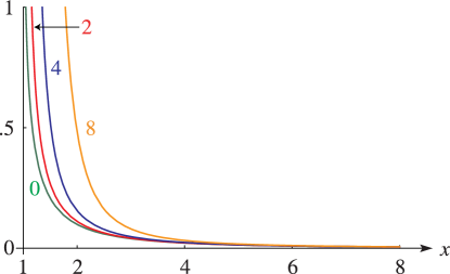
… ►Minimax polynomial approximations (§3.11(i)) for $K\left(k\right)$ and $E\left(k\right)$ in terms of $m=k^2$ with can be found in Abramowitz and Stegun (1964, §17.3) with maximum absolute errors ranging from 4×10⁻⁵ to 2×10⁻⁸. Approximations of the same type for $K\left(k\right)$ and $E\left(k\right)$ for are given in Cody (1965a) with maximum absolute errors ranging from 4×10⁻⁵ to 4×10⁻¹⁸. …

26: 29.7 Asymptotic Expansions

… ►

29.7.4 $${\tau }_1=\frac{p}{2^6}({(1+k^2)}^2(p^2+3)-4k^2(p^2+5)).$$

ⓘ

Symbols:

$p$: nonnegative integer, $k$: real parameter and ${\tau }_j$: coefficients

Permalink:

http://dlmf.nist.gov/29.7.E4

Encodings:

pMML, png, TeX

See also:

Annotations for §29.7(i), §29.7 and Ch.29

… ►

29.7.6 $${\tau }_2=\frac{1}{2^{10}}(1+k^2){(1-k^2)}^2(5p^4+34p^2+9),$$

ⓘ

Symbols:

$p$: nonnegative integer, $k$: real parameter and ${\tau }_j$: coefficients

Permalink:

http://dlmf.nist.gov/29.7.E6

Encodings:

pMML, png, TeX

See also:

Annotations for §29.7(i), §29.7 and Ch.29

►

29.7.7 $${\tau }_3=\frac{p}{2^{14}}({(1+k^2)}^4(33p^4+410p^2+405)-24k^2{(1+k^2)}^2(7p^4+90p^2+95)+16k^4(9p^4+130p^2+173)),$$

ⓘ

Symbols:

$p$: nonnegative integer, $k$: real parameter and ${\tau }_j$: coefficients

Permalink:

http://dlmf.nist.gov/29.7.E7

Encodings:

pMML, png, TeX

See also:

Annotations for §29.7(i), §29.7 and Ch.29

►

29.7.8 $${\tau }_4=\frac{1}{2^{16}}({(1+k^2)}^5(63p^6+1260p^4+2943p^2+486)-8k^2{(1+k^2)}^3(49p^6+1010p^4+2493p^2+432)+16k^4(1+k^2)(35p^6+760p^4+2043p^2+378)).$$

ⓘ

Symbols:

$p$: nonnegative integer, $k$: real parameter and ${\tau }_j$: coefficients

Permalink:

http://dlmf.nist.gov/29.7.E8

Encodings:

pMML, png, TeX

See also:

Annotations for §29.7(i), §29.7 and Ch.29

…

27: 4.24 Inverse Trigonometric Functions: Further Properties

… ►

4.24.1 $$\arcsin z=z+\frac{1}{2}\frac{z^3}{3}+\frac{1\cdot 3}{2\cdot 4}\frac{z^5}{5}+\frac{1\cdot 3\cdot 5}{2\cdot 4\cdot 6}\frac{z^7}{7}+\mathrm{\cdots },$$ $|z|\le 1$.

ⓘ

Symbols:

$\arcsin z$: arcsine function and $z$: complex variable

A&S Ref:

4.4.40 (where the constraint is .)

Permalink:

http://dlmf.nist.gov/4.24.E1

Encodings:

pMML, png, TeX

See also:

Annotations for §4.24(i), §4.24 and Ch.4

… ►

4.24.5 $$\arctan z=\frac{z}{z^2+1}\left(1+\frac{2}{3}\frac{z^2}{1+z^2}+\frac{2\cdot 4}{3\cdot 5}{\left(\frac{z^2}{1+z^2}\right)}^2+\mathrm{\cdots }\right),$$ $\mathrm{\Re }\left(z^2\right)>-\frac{1}{2}$,

ⓘ

Symbols:

$\arctan z$: arctangent function, $\mathrm{\Re }$: real part and $z$: complex variable

A&S Ref:

4.4.42 (has an error in the conditions on $z$.)

Permalink:

http://dlmf.nist.gov/4.24.E5

Encodings:

pMML, png, TeX

See also:

Annotations for §4.24(i), §4.24 and Ch.4

…

28: 3.4 Differentiation

… ►

$B_{-1}^4=-\frac{1}{6}(4-8t-3t^2+4t^3),$

… ►

$B_1^4=\frac{1}{6}(4+8t-3t^2-4t^3),$

… ►

$$B_0^5=-\frac{1}{12}(4+30t-15t^2-12t^3+5t^4),$$

… ►

$$B_3^5=\frac{1}{120}(4-15t^2+5t^4).$$

… ►For additional formulas involving values of ${\nabla }^{2}u$ and ${\nabla }^{4}u$ on square, triangular, and cubic grids, see Collatz (1960, Table VI, pp. 542–546). …

29: 26.2 Basic Definitions

… ►If, for example, a permutation of the integers 1 through 6 is denoted by $256413$, then the cycles are $\left(1,2,5\right)$, $\left(3,6\right)$, and $\left(4\right)$. …The function $\sigma$ also interchanges 3 and 6, and sends 4 to itself. … ►As an example, $\{1,3,4\}$, $\{2,6\}$, $\{5\}$ is a partition of $\{1,2,3,4,5,6\}$. … ►As an example, $\{1,1,1,2,4,4\}$ is a partition of 13. … ►The example $\{1,1,1,2,4,4\}$ has six parts, three of which equal 1. …

30: 27.15 Chinese Remainder Theorem

… ►Choose four relatively prime moduli $m_1,m_2,m_3$, and $m_4$ of five digits each, for example $2^{16}-3$, $2^{16}-1$, $2^{16}+1$, and $2^{16}+3$. …By the Chinese remainder theorem each integer in the data can be uniquely represented by its residues (mod $m_1$), (mod $m_2$), (mod $m_3$), and (mod $m_4$), respectively. Because each residue has no more than five digits, the arithmetic can be performed efficiently on these residues with respect to each of the moduli, yielding answers $a_1(mod{m}_1)$, $a_2(mod{m}_2)$, $a_3(mod{m}_3)$, and $a_4(mod{m}_4)$, where each $a_j$ has no more than five digits. …