of%20imaginary%20argument

SearchAdvancedHelp

(0.002 seconds)

1—10 of 12 matching pages

1: 5.22 Tables

… ►Abramowitz and Stegun (1964, Chapter 6) tabulates $\mathrm{\Gamma }\left(x\right)$, $\ln \mathrm{\Gamma }\left(x\right)$, $\psi \left(x\right)$, and ${\psi }^{\prime }\left(x\right)$ for $x=1(.005)2$ to 10D; ${\psi }^{\prime \prime }\left(x\right)$ and ${\psi }^{(3)}\left(x\right)$ for $x=1(.01)2$ to 10D; $\mathrm{\Gamma }\left(n\right)$, $1/\mathrm{\Gamma }\left(n\right)$, $\mathrm{\Gamma }\left(n+\frac{1}{2}\right)$, $\psi \left(n\right)$, ${\log }_{10}\mathrm{\Gamma }\left(n\right)$, ${\log }_{10}\mathrm{\Gamma }\left(n+\frac{1}{3}\right)$, ${\log }_{10}\mathrm{\Gamma }\left(n+\frac{1}{2}\right)$, and ${\log }_{10}\mathrm{\Gamma }\left(n+\frac{2}{3}\right)$ for $n=1(1)101$ to 8–11S; $\mathrm{\Gamma }\left(n+1\right)$ for $n=100(100)1000$ to 20S. … ►Abramov (1960) tabulates $\ln \mathrm{\Gamma }\left(x+\mathrm{i}y\right)$ for $x=1$ ($.01$) $2$, $y=0$ ($.01$) $4$ to 6D. Abramowitz and Stegun (1964, Chapter 6) tabulates $\ln \mathrm{\Gamma }\left(x+\mathrm{i}y\right)$ for $x=1$ ($.1$) $2$, $y=0$ ($.1$) $10$ to 12D. This reference also includes $\psi \left(x+\mathrm{i}y\right)$ for the same arguments to 5D. Zhang and Jin (1996, pp. 70, 71, and 73) tabulates the real and imaginary parts of $\mathrm{\Gamma }\left(x+\mathrm{i}y\right)$, $\ln \mathrm{\Gamma }\left(x+\mathrm{i}y\right)$, and $\psi \left(x+\mathrm{i}y\right)$ for $x=0.5,1,5,10$, $y=0(.5)10$ to 8S.

2: Software Index

… ► ►►►►►►►

	Open Source													With Book						Commercial
…
10.77(vi) Bessel Functions–Imaginary Order and Real Argument	✓	✓										✓	✓								✓	✓	✓
…
16.27(ii) Real Arguments	✓		✓		✓	✓						a	✓								✓	✓	✓
16.27(iii) Complex Arguments	✓											a	✓								✓	✓	✓
…
20 Theta Functions
…
22.22(ii) Real Argument	✓		✓		✓	✓		✓				✓	✓	✓		✓	✓		✓	✓	✓	✓	✓	✓
…

…

3: Bibliography B

… ►

Pionic atoms. Annual Review of Nuclear and Particle Science 20, pp. 467–508.

ⓘ

External Links:

Document

Referenced by:

§33.22(iv).

Encodings:

BibTeX

… ►

A program for computing the Riemann zeta function for complex argument. Comput. Phys. Comm. 20 (3), pp. 441–445.

ⓘ

Notes:

Double-precision Fortran, maximum accuracy 10S.

External Links:

Document, Code, ZentralBlatt

Referenced by:

1st item.

Encodings:

BibTeX

… ►

Evaluation of the incomplete gamma function of imaginary argument by Chebyshev polynomials. Math. Comp. 15 (73), pp. 7–11.

ⓘ

External Links:

FullText, MathReview (J. C. P. Miller), ZentralBlatt

Referenced by:

§8.7.

Encodings:

BibTeX

… ►

Coulomb functions (negative energies). Comput. Phys. Comm. 20 (3), pp. 447–458.

ⓘ

Notes:

Double-precision Fortran code.

External Links:

Document, Code

Referenced by:

1st item, 4th item.

Encodings:

BibTeX

… ►

Generalized hypergeometric functions at unit argument. Proc. Amer. Math. Soc. 114 (1), pp. 145–153.

ⓘ

External Links:

ISSN 0002-9939, FullText, MathReview (R. K. Raina), ZentralBlatt

Referenced by:

§16.4(ii), §16.8(ii).

Encodings:

BibTeX

…

4: Bibliography D

… ►

Complex zeros of cylinder functions. Math. Comp. 20 (94), pp. 215–222.

ⓘ

Notes:

For a numerical error in one of the zeros see Amos (1985).

External Links:

ISSN 0025-5718, FullText, MathReview, ZentralBlatt

Referenced by:

2nd item.

Encodings:

BibTeX

… ►

Bessel functions $J_n(z)$ and $Y_n(z)$ of integer order and complex argument. Comput. Phys. Comm. 78 (1-2), pp. 181–189.

ⓘ

Notes:

Double-precision Pascal, maximum accuracy 7D.

External Links:

ISSN 0010-4655, Document, Code, MathReview (J. P. Singhal), ZentralBlatt

Referenced by:

2nd item.

Encodings:

BibTeX

… ►

Uniform asymptotic expansions for Whittaker’s confluent hypergeometric functions. SIAM J. Math. Anal. 20 (3), pp. 744–760.

ⓘ

Notes:

(This reference has several typographical errors.)

External Links:

ISSN 0036-1410, Document, MathReview (F. W. J. Olver), ZentralBlatt

Referenced by:

§13.21(ii), §13.21(iii), §13.21(iv).

Encodings:

BibTeX

►

Bessel functions of purely imaginary order, with an application to second-order linear differential equations having a large parameter. SIAM J. Math. Anal. 21 (4), pp. 995–1018.

ⓘ

Notes:

Errata: In eq. (2.8) replace ${(x^2/4)}^2$ by ${(x^2/4)}^s$. In eq. (4.2) $\varphi (\zeta )$ should be replaced by $\psi (\zeta )$. In the second line of eq. (4.7) insert an external factor $e^{-2\pi ij/3}$ and change the upper limit of the sum to $n-1$. In eq. (4.15) the factor $\zeta$ is missing from the arguments of the functions Bi_ν and Bi’_ν.

External Links:

ISSN 0036-1410, Document, MathReview (A. de Castro Brzezicki), ZentralBlatt

Referenced by:

§10.24, §10.45, §2.8(iv).

Encodings:

BibTeX

… ►

Conical functions of purely imaginary order and argument. Proc. Roy. Soc. Edinburgh Sect. A 143 (5), pp. 929–955.

ⓘ

External Links:

ISSN 0308-2105, Document, Link, MathReview (Eugenia N. Petropoulou), ZentralBlatt

Referenced by:

§14.20(ix), §14.20(ix).

Encodings:

BibTeX

…

5: 20.10 Integrals

… ►

20.10.1 $${\int }_0^{\mathrm{\infty }}{x}^{s-1}{\theta }_2\left(0\right|\mathrm{i}{x}^2)dx=2^s(1-2^{-s}){\pi }^{-s/2}\mathrm{\Gamma }\left(\frac{1}{2}s\right)\zeta \left(s\right),$$ $\mathrm{\Re }s>1$,

ⓘ

Symbols:

$\mathrm{\Gamma }\left(z\right)$: gamma function, ${\theta }_j\left(z\right|\tau )$: theta function, $\zeta \left(s\right)$: Riemann zeta function, $\pi$: the ratio of the circumference of a circle to its diameter, $dx$: differential of $x$ , $\mathrm{i}$: imaginary unit, $\int$: integral and $\mathrm{\Re }$: real part

Keywords:

Mellin transform

Referenced by:

§20.10(i), Erratum (V1.1.5) for §20.10(i)

Permalink:

http://dlmf.nist.gov/20.10.E1

Encodings:

pMML, png, TeX

Modification (effective with 1.1.5):

Originally the constraint was $\mathrm{\Re }s>2$. This can be relaxed to $\mathrm{\Re }s>1$ because ${\theta }_2\left(0\right|\mathrm{i}{x}^2)=x^{-1}{\theta }_4\left(0\right|\mathrm{i}{x}^{-2})\sim x^{-1}$ as $x\to 0+$, which follows from (20.7.31) and (20.4.5).

See also:

Annotations for §20.10(i), §20.10 and Ch.20

►

20.10.2 $${\int }_0^{\mathrm{\infty }}{x}^{s-1}({\theta }_3\left(0\right|\mathrm{i}{x}^2)-1)dx={\pi }^{-s/2}\mathrm{\Gamma }\left(\frac{1}{2}s\right)\zeta \left(s\right),$$ $\mathrm{\Re }s>1$,

ⓘ

Symbols:

$\mathrm{\Gamma }\left(z\right)$: gamma function, ${\theta }_j\left(z\right|\tau )$: theta function, $\zeta \left(s\right)$: Riemann zeta function, $\pi$: the ratio of the circumference of a circle to its diameter, $dx$: differential of $x$ , $\mathrm{i}$: imaginary unit, $\int$: integral and $\mathrm{\Re }$: real part

Keywords:

Mellin transform

Referenced by:

§20.10(i), Erratum (V1.1.5) for §20.10(i)

Permalink:

http://dlmf.nist.gov/20.10.E2

Encodings:

pMML, png, TeX

Modification (effective with 1.1.5):

Originally the constraint was $\mathrm{\Re }s>2$. This can be relaxed to $\mathrm{\Re }s>1$ because ${\theta }_3\left(0\right|\mathrm{i}{x}^2)=x^{-1}{\theta }_3\left(0\right|\mathrm{i}{x}^{-2})\sim x^{-1}$ as $x\to 0+$, which follows from (20.7.32) and (20.4.4).

See also:

Annotations for §20.10(i), §20.10 and Ch.20

►

20.10.3 $${\int }_0^{\mathrm{\infty }}{x}^{s-1}(1-{\theta }_4\left(0\right|\mathrm{i}{x}^2))dx=(1-2^{1-s}){\pi }^{-s/2}\mathrm{\Gamma }\left(\frac{1}{2}s\right)\zeta \left(s\right),$$ $\mathrm{\Re }s>0$.

ⓘ

Symbols:

$\mathrm{\Gamma }\left(z\right)$: gamma function, ${\theta }_j\left(z\right|\tau )$: theta function, $\zeta \left(s\right)$: Riemann zeta function, $\pi$: the ratio of the circumference of a circle to its diameter, $dx$: differential of $x$ , $\mathrm{i}$: imaginary unit, $\int$: integral and $\mathrm{\Re }$: real part

Keywords:

Mellin transform

Referenced by:

§20.10(i), Erratum (V1.1.5) for §20.10(i)

Permalink:

http://dlmf.nist.gov/20.10.E3

Encodings:

pMML, png, TeX

Modification (effective with 1.1.5):

Originally the constraint was $\mathrm{\Re }s>2$. This can be relaxed to $\mathrm{\Re }s>0$ because $1-{\theta }_4\left(0\right|\mathrm{i}{x}^2)=1-x^{-1}{\theta }_2\left(0\right|\mathrm{i}{x}^{-2})\sim 1$ as $x\to 0+$, which follows from (20.7.33) and (20.4.3).

See also:

Annotations for §20.10(i), §20.10 and Ch.20

… ►Let $s$, $\mathrm{\ell }$, and $\beta$ be constants such that $\mathrm{\Re }s>0$, $\mathrm{\ell }>0$, and $\left|\mathrm{\Re }\beta \right|+\left|\mathrm{\Im }\beta \right|\le \mathrm{\ell }$. … ►For corresponding results for argument derivatives of the theta functions see Erdélyi et al. (1954a, pp. 224–225) or Oberhettinger and Badii (1973, p. 193). …

6: 9.18 Tables

… ►

Miller (1946) tabulates $\mathrm{Ai}\left(x\right)$, ${\mathrm{Ai}}^{\prime }\left(x\right)$ for $x=-20(.01)2;$ ${\log }_{10}\mathrm{Ai}\left(x\right)$, ${\mathrm{Ai}}^{\prime }\left(x\right)/\mathrm{Ai}\left(x\right)$ for $x=0(.1)25(1)75$; $\mathrm{Bi}\left(x\right)$, ${\mathrm{Bi}}^{\prime }\left(x\right)$ for $x=-10(.1)2.5$; ${\log }_{10}\mathrm{Bi}\left(x\right)$, ${\mathrm{Bi}}^{\prime }\left(x\right)/\mathrm{Bi}\left(x\right)$ for $x=0(.1)10$; $M\left(x\right)$, $N\left(x\right)$, $\theta \left(x\right)$, $\varphi \left(x\right)$ (respectively $F(x)$, $G(x)$, $\chi (x)$, $\psi (x)$) for $x=-80(1)-30(.1)0$. Precision is generally 8D; slightly less for some of the auxiliary functions. Extracts from these tables are included in Abramowitz and Stegun (1964, Chapter 10), together with some auxiliary functions for large arguments.

… ►

Zhang and Jin (1996, p. 337) tabulates $\mathrm{Ai}\left(x\right)$, ${\mathrm{Ai}}^{\prime }\left(x\right)$, $\mathrm{Bi}\left(x\right)$, ${\mathrm{Bi}}^{\prime }\left(x\right)$ for $x=0(1)20$ to 8S and for $x=-20(1)0$ to 9D.

… ►

Miller (1946) tabulates $a_k$, ${\mathrm{Ai}}^{\prime }\left(a_k\right)$, $a_k^{\prime }$, $\mathrm{Ai}\left(a_k^{\prime }\right)$, $k=1(1)50$; $b_k$, ${\mathrm{Bi}}^{\prime }\left(b_k\right)$, $b_k^{\prime }$, $\mathrm{Bi}\left(b_k^{\prime }\right)$, $k=1(1)20$. Precision is 8D. Entries for $k=1(1)20$ are reproduced in Abramowitz and Stegun (1964, Chapter 10).

►

Sherry (1959) tabulates $a_k$, ${\mathrm{Ai}}^{\prime }\left(a_k\right)$, $a_k^{\prime }$, $\mathrm{Ai}\left(a_k^{\prime }\right)$, $k=1(1)50$; 20S.

… ►

Corless et al. (1992) gives the real and imaginary parts of ${\beta }_k$ for $k=1(1)13$; 14S.

…

7: Bibliography G

… ►

Algorithm 259: Legendre functions for arguments larger than one. Comm. ACM 8 (8), pp. 488–492.

ⓘ

Notes:

Variable-precision Algol. For remark see ACM Trans. Math. Software 3(2) (1977), p. 204–205

External Links:

ISSN 0001-0782, Document

Referenced by:

§14.34(ii).

Encodings:

BibTeX

… ►

Some integrals involving three Bessel functions when their arguments satisfy the triangle inequalities. J. Math. Phys. 25 (11), pp. 3350–3356.

ⓘ

External Links:

ISSN 0022-2488, Document, MathReview (B. R. Bhonsle), ZentralBlatt

Referenced by:

§10.22(iv), §10.43(iv).

Encodings:

BibTeX

… ►

Algorithm 831: Modified Bessel functions of imaginary order and positive argument. ACM Trans. Math. Software 30 (2), pp. 159–164.

ⓘ

External Links:

ISSN 0098-3500, Document, GAMS (module 831; package TOMS), MathReview Entry, ZentralBlatt

Referenced by:

1st item.

Encodings:

BibTeX

►

Computing solutions of the modified Bessel differential equation for imaginary orders and positive arguments. ACM Trans. Math. Software 30 (2), pp. 145–158.

ⓘ

External Links:

ISSN 0098-3500, Document, MathReview, ZentralBlatt

Referenced by:

§10.74(viii).

Encodings:

BibTeX

… ►

Algorithm 939: computation of the Marcum Q-function. ACM Trans. Math. Softw. 40 (3), pp. 20:1–20:21.

ⓘ

Notes:

Includes Fortran program claiming 12S accuracy

External Links:

ISSN 0098-3500, Link, Document, MathReview Entry, ZentralBlatt

Referenced by:

3rd item, §10.77(ix).

Encodings:

BibTeX

…

8: 22.3 Graphics

… ► $\mathrm{sn}(x,k)$, $\mathrm{cn}(x,k)$, and $\mathrm{dn}(x,k)$ as functions of real arguments $x$ and $k$. … ►

►►

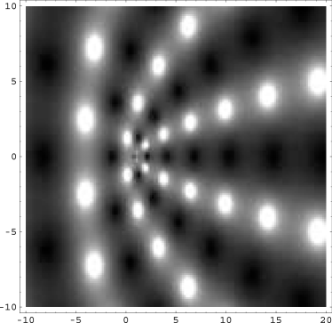
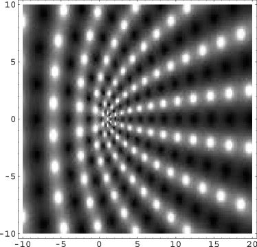
Figure 22.3.26: Density plot of $|\mathrm{sn}(5,k)|$ as a function of complex $k^2$, $-10\le \mathrm{\Re }\left(k^2\right)\le 20$, $-10\le \mathrm{\Im }\left(k^2\right)\le 10$. … Magnify

►

►►

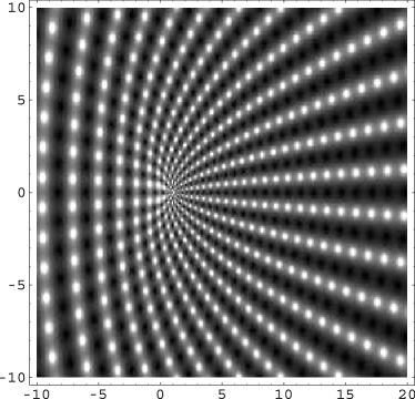
Figure 22.3.27: Density plot of $|\mathrm{sn}(10,k)|$ as a function of complex $k^2$, $-10\le \mathrm{\Re }\left(k^2\right)\le 20$, $-10\le \mathrm{\Im }\left(k^2\right)\le 10$. … Magnify

►

►►

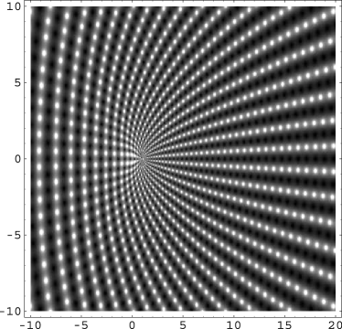
Figure 22.3.28: Density plot of $|\mathrm{sn}(20,k)|$ as a function of complex $k^2$, $-10\le \mathrm{\Re }\left(k^2\right)\le 20$, $-10\le \mathrm{\Im }\left(k^2\right)\le 10$. … Magnify

►

►►

Figure 22.3.29: Density plot of $|\mathrm{sn}(30,k)|$ as a function of complex $k^2$, $-10\le \mathrm{\Re }\left(k^2\right)\le 20$, $-10\le \mathrm{\Im }\left(k^2\right)\le 10$. … Magnify

9: 20.11 Generalizations and Analogs

… ►

20.11.1 $$G(m,n)=\sum _{k=0}^{n-1}{\mathrm{e}}^{-\pi \mathrm{i}{k}^{2}m/n};$$

ⓘ

Defines:

$G(m,n)$: Gauss sum (locally)

Symbols:

$\pi$: the ratio of the circumference of a circle to its diameter, $\mathrm{e}$: base of natural logarithm, $\mathrm{i}$: imaginary unit, $m$: integer and $n$: integer

Permalink:

http://dlmf.nist.gov/20.11.E1

Encodings:

pMML, png, TeX

See also:

Annotations for §20.11(i), §20.11 and Ch.20

… ►If both $m,n$ are positive, then $G(m,n)$ allows inversion of its arguments as a modular transformation (compare (23.15.3) and (23.15.4)): ►

20.11.2 $$\frac{1}{\sqrt{n}}G(m,n)=\frac{1}{\sqrt{n}}\sum _{k=0}^{n-1}{\mathrm{e}}^{-\pi \mathrm{i}{k}^{2}m/n}=\frac{{\mathrm{e}}^{-\pi \mathrm{i}/4}}{\sqrt{m}}\sum _{j=0}^{m-1}{\mathrm{e}}^{\pi \mathrm{i}{j}^{2}n/m}=\frac{{\mathrm{e}}^{-\pi \mathrm{i}/4}}{\sqrt{m}}G(-n,m).$$

ⓘ

Symbols:

$\pi$: the ratio of the circumference of a circle to its diameter, $\mathrm{e}$: base of natural logarithm, $\mathrm{i}$: imaginary unit, $m$: integer, $n$: integer and $G(m,n)$: Gauss sum

Permalink:

http://dlmf.nist.gov/20.11.E2

Encodings:

pMML, png, TeX

See also:

Annotations for §20.11(i), §20.11 and Ch.20

… ►With the substitutions $a=q{\mathrm{e}}^{2\mathrm{i}z}$, $b=q{\mathrm{e}}^{-2\mathrm{i}z}$, with $q={\mathrm{e}}^{\mathrm{i}\pi \tau }$, we have …

10: 25.6 Integer Arguments

§25.6 Integer Arguments

►

§25.6(i) Function Values

… ►

25.6.3 $$\zeta \left(-n\right)=-\frac{B_{n+1}}{n+1},$$ $n=1,2,3,\mathrm{\dots }$.

ⓘ

Symbols:

$B_n$: Bernoulli numbers, $\zeta \left(s\right)$: Riemann zeta function and $n$: nonnegative integer

Source:

Apostol (1976, (20), p. 266); with $n\ne 0$

A&S Ref:

23.2.15 (in slightly different form)

Permalink:

http://dlmf.nist.gov/25.6.E3

Encodings:

pMML, png, TeX

See also:

Annotations for §25.6(i), §25.6 and Ch.25

… ►

§25.6(ii) Derivative Values

… ►

25.6.13 $${(-1)}^k{\zeta }^{(k)}\left(-2n\right)=\frac{2{(-1)}^n}{{(2\pi )}^{2n+1}}\sum _{m=0}^k\sum _{r=0}^m\left(\genfrac{}{}{0.0pt}{}{k}{m}\right)\left(\genfrac{}{}{0.0pt}{}{m}{r}\right)\mathrm{\Im }\left(c^{k-m}\right){\mathrm{\Gamma }}^{(r)}\left(2n+1\right){\zeta }^{(m-r)}\left(2n+1\right),$$

ⓘ

Symbols:

$\mathrm{\Gamma }\left(z\right)$: gamma function, $\zeta \left(s\right)$: Riemann zeta function, $\left(\genfrac{}{}{0.0pt}{}{m}{n}\right)$: binomial coefficient, $\pi$: the ratio of the circumference of a circle to its diameter, $\mathrm{\Im }$: imaginary part, $k$: nonnegative integer, $m$: nonnegative integer, $n$: nonnegative integer and $c$

Source:

Apostol (1985a, p. 225)

Permalink:

http://dlmf.nist.gov/25.6.E13

Encodings:

pMML, png, TeX

See also:

Annotations for §25.6(ii), §25.6 and Ch.25

…