computation of coefficients

SearchAdvancedHelp

(0.002 seconds)

31—40 of 56 matching pages

31: 10.75 Tables

… ►

Olver (1962) provides tables for the uniform asymptotic expansions given in §10.20(i), including $\zeta$ and ${(4\zeta /(1-x^2))}^{\frac{1}{4}}$ as functions of $x$ $(=z)$ and the coefficients $A_k(\zeta )$, $B_k(\zeta )$, $C_k(\zeta )$, $D_k(\zeta )$ as functions of $\zeta$. These enable $J_{\nu }\left(\nu x\right)$, $Y_{\nu }\left(\nu x\right)$, $J_{\nu }^{\prime }\left(\nu x\right)$, $Y_{\nu }^{\prime }\left(\nu x\right)$ to be computed to 10S when $\nu \ge 15$, except in the neighborhoods of zeros.

… ►

Olver (1962) provides tables for the uniform asymptotic expansions given in §10.41(ii), including $\eta$ and the coefficients $U_k(p)$, $V_k(p)$ as functions of $p={(1+x^2)}^{-\frac{1}{2}}$. These enable $I_{\nu }\left(\nu x\right)$, $K_{\nu }\left(\nu x\right)$, $I_{\nu }^{\prime }\left(\nu x\right)$, $K_{\nu }^{\prime }\left(\nu x\right)$ to be computed to 10S when $\nu \ge 16$.

…

32: 23.22 Methods of Computation

§23.22 Methods of Computation

… ►The functions $\zeta \left(z\right)$ and $\sigma \left(z\right)$ are computed in a similar manner: the former by replacing $u$ and $z$ in (23.6.13) by $z$ and $\pi z/(2{\omega }_1)$, respectively, and also referring to (23.6.8); the latter by applying (23.6.9). … ► ►

§23.22(ii) Lattice Calculations

… ►Suppose that the invariants $g_2=c$, $g_3=d$, are given, for example in the differential equation (23.3.10) or via coefficients of an elliptic curve (§23.20(ii)). …

33: Bibliography J

… ►

Further results on the computation of incomplete gamma functions. In Analytic Theory of Continued Fractions, II (Pitlochry/Aviemore, 1985), W. J. Thron (Ed.), Lecture Notes in Math. 1199, pp. 67–89.

ⓘ

External Links:

MathReview (Marietta J. Tretter), ZentralBlatt

Referenced by:

§8.25(iv).

Encodings:

BibTeX

… ►

Monodromy preserving deformation of linear ordinary differential equations with rational coefficients. II. Phys. D 2 (3), pp. 407–448.

ⓘ

External Links:

ISSN 0167-2789, Document, MathReview (V. A. Golubeva), ZentralBlatt

Referenced by:

§32.4(i), §32.4(ii), §32.4(iv), §32.4(v), §32.6(ii), §32.6(iii), §32.6(iv), §32.6(v), §32.6(v), §32.6(v).

Encodings:

BibTeX

… ►

Efficient implementation of the Hardy-Ramanujan-Rademacher formula. LMS J. Comput. Math. 15, pp. 341–359.

ⓘ

External Links:

ISSN 1461-1570, Document, Link, MathReview (Tim Huber), ZentralBlatt

Referenced by:

§27.20.

Encodings:

BibTeX

… ►

Parabolic cylinder functions of large order. J. Comput. Appl. Math. 190 (1-2), pp. 453–469.

ⓘ

External Links:

ISSN 0377-0427, Document, MathReview Entry, ZentralBlatt

Referenced by:

§12.10(vi).

Encodings:

BibTeX

… ►

On the computation of incomplete gamma functions in the complex domain. J. Comput. Appl. Math. 12/13, pp. 401–417.

ⓘ

External Links:

ISSN 0377-0427, Document, MathReview (M. Marsden), ZentralBlatt

Referenced by:

§8.25(iv), §8.9.

Encodings:

BibTeX

…

34: 30.18 Software

… ►A more complete list of available software for computing these functions is found in the Software Index. … ►

SWF7: Coefficients ${\beta }_p$ in (30.9.1).

►

SWF8: Coefficients $c_p$ in (30.9.4).

►

SWF9: Coefficients ${\mathrm{\ell }}_p$ in (30.3.8).

…

35: Bibliography W

… ►

Evaluating elliptic functions and their inverses. Comput. Math. Appl. 39 (3-4), pp. 131–136.

ⓘ

External Links:

ISSN 0898-1221, Document, MathReview, ZentralBlatt

Referenced by:

§22.20(ii), §22.20(v).

Encodings:

BibTeX

… ►

Computation of the Whittaker function of the second kind by summing its divergent asymptotic series with the help of nonlinear sequence transformations. Computers in Physics 10 (5), pp. 496–503.

ⓘ

External Links:

Document

Referenced by:

§2.11(vi), §2.11(vi).

Encodings:

BibTeX

… ►

Computation with Recurrence Relations. Pitman, Boston, MA.

ⓘ

External Links:

ISBN 0-273-08508-5, MathReview (S. Conde), ZentralBlatt

Referenced by:

§13.29(iv), §16.25, §2.9(iii), §3.10(iii), §3.6(iii), §3.6(v), §3.6(vii).

Encodings:

BibTeX

… ►

Algorithm 44: Bessel functions computed recursively. Comm. ACM 4 (4), pp. 177–178.

ⓘ

Notes:

Includes Algol code, maximum accuracy 8S.

External Links:

ISSN 0001-0782, Document

Referenced by:

§10.77(ii).

Encodings:

BibTeX

… ►

On the asymptotic behavior of the Fourier coefficients of Mathieu functions. J. Res. Nat. Inst. Standards Tech. 113 (1), pp. 11–15.

ⓘ

External Links:

ISSN 1044-677X, FullText

Referenced by:

§28.4(vii).

Encodings:

BibTeX

…

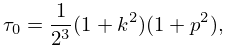
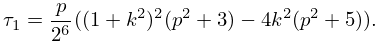
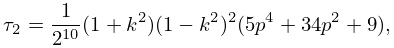
36: 10.21 Zeros

… ►For the first zeros rounded numerical values of the coefficients are given by … ►For numerical coefficients for $m=2,3,4,5$ see Olver (1951, Tables 3–6). … ►The latter reference includes numerical tables of the first few coefficients in the uniform asymptotic expansions. … ►Higher coefficients in the asymptotic expansions in this subsection can be obtained by expressing the cross-products in terms of the modulus and phase functions (§10.18), and then reverting the asymptotic expansion for the difference of the phase functions. … ►For properties, computation, and generalizations see Kapitsa (1951b), Kerimov (1999, 2008), and Gupta and Muldoon (2000). …

37: 3.5 Quadrature

… ►which depends on function values computed previously. … ►can be computed by Filon’s rule. … ►

Example

… ► … ► …

38: 29.7 Asymptotic Expansions

… ►

29.7.1 $$a_{\nu }^m\left(k^2\right)\sim p\kappa -{\tau }_0-{\tau }_1{\kappa }^{-1}-{\tau }_2{\kappa }^{-2}-\mathrm{\cdots },$$

ⓘ

Symbols:

$a_{\nu }^n\left(k^2\right)$: eigenvalues of Lamé’s equation, $\sim$: Poincaré asymptotic expansion, $m$: nonnegative integer, $p$: nonnegative integer, $k$: real parameter, $\nu$: real parameter, $\kappa$ and ${\tau }_j$: coefficients

Permalink:

http://dlmf.nist.gov/29.7.E1

Encodings:

pMML, png, TeX

See also:

Annotations for §29.7(i), §29.7 and Ch.29

… ►

29.7.3 $${\tau }_0=\frac{1}{2^3}(1+k^2)(1+p^2),$$

ⓘ

Symbols:

$p$: nonnegative integer, $k$: real parameter and ${\tau }_j$: coefficients

Permalink:

http://dlmf.nist.gov/29.7.E3

Encodings:

pMML, png, TeX

See also:

Annotations for §29.7(i), §29.7 and Ch.29

►

29.7.4 $${\tau }_1=\frac{p}{2^6}({(1+k^2)}^2(p^2+3)-4k^2(p^2+5)).$$

ⓘ

Symbols:

$p$: nonnegative integer, $k$: real parameter and ${\tau }_j$: coefficients

Permalink:

http://dlmf.nist.gov/29.7.E4

Encodings:

pMML, png, TeX

See also:

Annotations for §29.7(i), §29.7 and Ch.29

… ►

29.7.6 $${\tau }_2=\frac{1}{2^{10}}(1+k^2){(1-k^2)}^2(5p^4+34p^2+9),$$

ⓘ

Symbols:

$p$: nonnegative integer, $k$: real parameter and ${\tau }_j$: coefficients

Permalink:

http://dlmf.nist.gov/29.7.E6

Encodings:

pMML, png, TeX

See also:

Annotations for §29.7(i), §29.7 and Ch.29

… ►Formulas for additional terms can be computed with the author’s Maple program LA5; see §29.22. …

39: 3.8 Nonlinear Equations

§3.8 Nonlinear Equations

… ►All zeros of $f$ in the original interval $[a,b]$ can be computed to any predetermined accuracy. … ►

§3.8(iv) Zeros of Polynomials

… ►However, when the coefficients are all real, complex arithmetic can be avoided by the following iterative process. … ►For further information on the computation of zeros of polynomials see McNamee (2007). …

40: 26.6 Other Lattice Path Numbers

… ►

26.6.1 $$D(m,n)=\sum _{k=0}^n\left(\genfrac{}{}{0.0pt}{}{n}{k}\right)\left(\genfrac{}{}{0.0pt}{}{m+n-k}{n}\right)=\sum _{k=0}^n{2}^k\left(\genfrac{}{}{0.0pt}{}{m}{k}\right)\left(\genfrac{}{}{0.0pt}{}{n}{k}\right).$$

ⓘ

Defines:

$D(m,n)$: Delannoy number (locally)

Symbols:

$\left(\genfrac{}{}{0.0pt}{}{m}{n}\right)$: binomial coefficient, $k$: nonnegative integer, $m$: nonnegative integer and $n$: nonnegative integer

Permalink:

http://dlmf.nist.gov/26.6.E1

Encodings:

pMML, png, TeX

See also:

Annotations for §26.6(i), §26.6(i), §26.6 and Ch.26

… ►

26.6.2 $$M(n)=\sum _{k=0}^n\frac{{(-1)}^k}{n+2-k}\left(\genfrac{}{}{0.0pt}{}{n}{k}\right)\left(\genfrac{}{}{0.0pt}{}{2n+2-2k}{n+1-k}\right).$$

ⓘ

Defines:

$M(n)$: Motzkin number (locally)

Symbols:

$\left(\genfrac{}{}{0.0pt}{}{m}{n}\right)$: binomial coefficient, $k$: nonnegative integer and $n$: nonnegative integer

Permalink:

http://dlmf.nist.gov/26.6.E2

Encodings:

pMML, png, TeX

See also:

Annotations for §26.6(i), §26.6(i), §26.6 and Ch.26

… ►

26.6.3 $$N(n,k)=\frac{1}{n}\left(\genfrac{}{}{0.0pt}{}{n}{k}\right)\left(\genfrac{}{}{0.0pt}{}{n}{k-1}\right).$$

ⓘ

Defines:

$N(n,k)$: Narayana number (locally)

Symbols:

$\left(\genfrac{}{}{0.0pt}{}{m}{n}\right)$: binomial coefficient, $k$: nonnegative integer and $n$: nonnegative integer

Permalink:

http://dlmf.nist.gov/26.6.E3

Encodings:

pMML, png, TeX

See also:

Annotations for §26.6(i), §26.6(i), §26.6 and Ch.26

… ►

26.6.13 $$M(n)=\sum _{k=0}^n{(-1)}^k\left(\genfrac{}{}{0.0pt}{}{n}{k}\right)C\left(n+1-k\right),$$

ⓘ

Symbols:

$C\left(n\right)$: Catalan number, $\left(\genfrac{}{}{0.0pt}{}{m}{n}\right)$: binomial coefficient, $k$: nonnegative integer, $n$: nonnegative integer and $M(n)$: Motzkin number

Permalink:

http://dlmf.nist.gov/26.6.E13

Encodings:

pMML, png, TeX

See also:

Annotations for §26.6(iv), §26.6 and Ch.26

►

26.6.14 $$C\left(n\right)=\sum _{k=0}^{2n}{(-1)}^k\left(\genfrac{}{}{0.0pt}{}{2n}{k}\right)M(2n-k).$$

ⓘ

Symbols:

$C\left(n\right)$: Catalan number, $\left(\genfrac{}{}{0.0pt}{}{m}{n}\right)$: binomial coefficient, $k$: nonnegative integer, $n$: nonnegative integer and $M(n)$: Motzkin number

Permalink:

http://dlmf.nist.gov/26.6.E14

Encodings:

pMML, png, TeX

See also:

Annotations for §26.6(iv), §26.6 and Ch.26