%E9%82%A3%E4%B8%8D%E5%8B%92%E6%96%AF%E7%BE%8E%E6%9C%AF%E5%AD%A6%E9%99%A2%20Electronic%20Engineering%20Degree%20Certificate%E3%80%90%E4%BB%BF%E8%AF%81 %E5%BE%AEfuk7778%E3%80%91f63D
(0.017 seconds)
11—20 of 785 matching pages
11: 14.17 Integrals
…
►
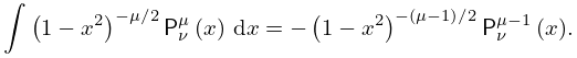
14.17.1
►
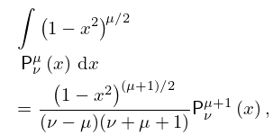
14.17.2
or .
►
14.17.3
.
…
►In (14.17.1)–(14.17.4), may be replaced by , and in (14.17.3) and (14.17.4), may be replaced by .
…
►For Mellin transforms involving associated Legendre functions see Oberhettinger (1974, pp. 69–82) and Marichev (1983, pp. 247–283), and for inverse transforms see Oberhettinger (1974, pp. 205–215).
12: 10.9 Integral Representations
…
►
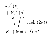
10.9.30
.
…
►For collections of integral representations of Bessel and Hankel functions see Erdélyi et al. (1953b, §§7.3 and 7.12), Erdélyi et al. (1954a, pp. 43–48, 51–60, 99–105, 108–115, 123–124, 272–276, and
356–357), Gröbner and Hofreiter (1950, pp. 189–192), Marichev (1983, pp. 191–192 and 196–210), Magnus et al. (1966, §3.6), and Watson (1944, Chapter 6).
13: Bibliography G
…
►
Positive sums of the classical orthogonal polynomials.
SIAM J. Math. Anal. 8 (3), pp. 423–447.
…
►
Algorithm 236: Bessel functions of the first kind.
Comm. ACM 7 (8), pp. 479–480.
►
Algorithm 259: Legendre functions for arguments larger than one.
Comm. ACM 8 (8), pp. 488–492.
…
►
Computational aspects of three-term recurrence relations.
SIAM Rev. 9 (1), pp. 24–82.
…
►
Analysis in homogeneous domains.
Uspehi Mat. Nauk 19 (4 (118)), pp. 3–92 (Russian).
…
14: 1.6 Vectors and Vector-Valued Functions
…
►Thus pairs of indefinite suffices in an expression are resolved by being summed over (or “traced” over).
…
►Note that can be given an orientation by means of .
…
►with , an open set in the plane.
…
►A surface is orientable if a continuously varying normal can be defined at all points of the surface.
…
►If and are both orientation preserving or both orientation reversing parametrizations of defined on open sets and respectively, then
…
15: Bibliography B
…
►
The generating function of Jacobi polynomials.
J. London Math. Soc. 13, pp. 8–12.
…
►
Cusped rainbows and incoherence effects in the rippling-mirror model for particle scattering from surfaces.
J. Phys. A 8 (4), pp. 566–584.
…
►
On the power function of the likelihood ratio test for MANOVA.
J. Multivariate Anal. 82 (2), pp. 416–421.
…
►
Angular Momentum in Quantum Physics: Theory and Application.
Encyclopedia of Mathematics and its Applications, Vol. 8, Addison-Wesley Publishing Co., Reading, M.A..
…
►
Algorithm 21: Bessel function for a set of integer orders.
Comm. ACM 3 (11), pp. 600.
…
16: Bibliography M
…
►
Inequalities for the zeros of Bessel functions.
SIAM J. Math. Anal. 8 (1), pp. 166–170.
…
►
Exact misclassification probabilities for plug-in normal quadratic discriminant functions. II. The heterogeneous case.
J. Multivariate Anal. 82 (2), pp. 299–330.
…
►
On the -function. VII, VIII.
Nederl. Akad. Wetensch., Proc. 49, pp. 1063–1072, 1165–1175 = Indagationes Math. 8, 661–670, 713–723 (1946).
…
►
Hierarchies and logarithmic oscillations in the temporal relaxation patterns of proteins and other complex systems.
Proc. Nat. Acad. Sci. U .S. A. 96 (20), pp. 11085–11089.
…
►
The characteristic numbers of the Mathieu equation with purely imaginary parameter.
Phil. Mag. Series 7 8 (53), pp. 834–840.
…
17: 10.21 Zeros
…
►The parameter may be regarded as a continuous variable and , as functions , of .
…
►Let , , and
be defined as in §10.21(ii) and , , , and denote the modulus and phase functions for the Airy functions and their derivatives as in §9.8.
…
►
and are defined by (10.20.11) and (10.20.12) with .
…
►Each curve that represents an infinite string of nonreal zeros should be located on the opposite side of its straight line asymptote.
…
►Higher coefficients in the asymptotic expansions in this subsection can be obtained by expressing the cross-products in terms of the modulus and phase functions (§10.18), and then reverting the asymptotic expansion for the difference of the phase functions.
…
18: Errata
…
►
Paragraph Prime Number Theorem (in §27.12)
…
►
Equation (10.19.11)
…
►
Table 26.8.1
…
►
Chapters 8, 20, 36
…
The largest known prime, which is a Mersenne prime, was updated from (2009) to (2018).
Version 1.0.11 (June 8, 2016)
… ►
10.19.11
Originally the first term on the right-hand side of this equation was written incorrectly as .
Reported 2015-03-16 by Svante Janson.
Originally the Stirling number was given incorrectly as 6327. The correct number is 63273.
| 10 | |||||||||||
Reported 2013-11-25 by Svante Janson.
