normalizing factor

SearchAdvancedHelp

(0.002 seconds)

1—10 of 15 matching pages

1: 3.6 Linear Difference Equations

… ►It therefore remains to apply a normalizing factor $\mathrm{\Lambda }$. … ►The normalizing factor $\mathrm{\Lambda }$ can be the true value of $w_0$ divided by its trial value, or $\mathrm{\Lambda }$ can be chosen to satisfy a known property of the wanted solution of the form … …

2: 3.7 Ordinary Differential Equations

… ►The eigenvalues ${\lambda }_k$ are simple, that is, there is only one corresponding eigenfunction (apart from a normalization factor), and when ordered increasingly the eigenvalues satisfy …

3: 18.39 Applications in the Physical Sciences

… ►All are written in the same form as the product of three factors: the square root of a weight function $w(x)$, the corresponding OP or EOP, and constant factors ensuring unit normalization. … ►With the normalization factor ${\left(c{h}_n\right)}^{-1/2}$ the ${\psi }_n$ are orthonormal in $L^2(ℝ,dx)$. …

4: 28.5 Second Solutions ${\mathrm{fe}}_n$, ${\mathrm{ge}}_n$

… ►The factors $C_n(q)$ and $S_n(q)$ in (28.5.1) and (28.5.2) are normalized so that ►

28.5.5 $${(C_n(q))}^2{\int }_0^{2\pi }{(f_n(x,q))}^{2}dx={(S_n(q))}^2{\int }_0^{2\pi }{(g_n(x,q))}^{2}dx=\pi .$$

ⓘ

Symbols:

$\pi$: the ratio of the circumference of a circle to its diameter, $dx$: differential of $x$ , $\int$: integral, $q=h^2$: parameter, $n$: integer, $x$: real variable, $f_n(z,q)$: functions, $g_n(z,q)$: functions, $C_n(q)$: factor and $S_n(q)$: factor

Permalink:

http://dlmf.nist.gov/28.5.E5

Encodings:

pMML, png, TeX

See also:

Annotations for §28.5(i), §28.5(i), §28.5 and Ch.28

…

5: 33.13 Complex Variable and Parameters

… ►

33.13.2 $$R_{\mathrm{\ell }}=(2\mathrm{\ell }+1)C_{\mathrm{\ell }}\left(\eta \right)/C_{\mathrm{\ell }-1}\left(\eta \right).$$

ⓘ

Symbols:

$C_{\mathrm{\ell }}\left(\eta \right)$: normalizing constant for Coulomb radial functions, $\mathrm{\ell }$: nonnegative integer, $\eta$: real parameter and $R_{\mathrm{\ell }}$: factor

Permalink:

http://dlmf.nist.gov/33.13.E2

Encodings:

pMML, png, TeX

See also:

Annotations for §33.13 and Ch.33

…

6: Bibliography C

… ►

Reduction theorems for elliptic integrands with the square root of two quadratic factors. J. Comput. Appl. Math. 118 (1-2), pp. 71–85.

ⓘ

Notes:

Code written by the second author to compute symmetric elliptic integrals numerically in the Derive computer algebra system is available.

External Links:

ISSN 0377-0427, Document, Code, MathReview, ZentralBlatt

Referenced by:

§19.29(ii), §19.36(i), §19.36(i), §19.39(iv).

Encodings:

BibTeX

… ►

Normal elliptic integrals of the first and second kinds. Duke Math. J. 31 (3), pp. 405–419.

ⓘ

External Links:

Document, MathReview (S. Hitotumatu), ZentralBlatt

Referenced by:

§19.22(iii), §19.23, §19.33(i), §19.33(i).

Encodings:

BibTeX

… ►

Demagnetization factors for general ellipsoids. J. Appl. Phys. 70 (6), pp. 2911–2914.

ⓘ

Notes:

For an erratum concerning availability of tables, see J. Appl. Phys 70(1991)7660.

External Links:

Document

Referenced by:

§19.15, §19.33(iii).

Encodings:

BibTeX

… ►

ⓘ

Notes:

Seeks to factor numbers of the form $b^n\pm 1$ for $b=2,3,5,6,7,10,11,12$.

External Links:

Home Page

Referenced by:

3rd item.

Encodings:

BibTeX

►

Algorithm AS 24: From normal integral to deviate. Appl. Statist. 18 (3), pp. 290–293.

ⓘ

Notes:

Includes Fortran program, maximum accuracy 12D.

External Links:

FullText

Referenced by:

§7.25(ii).

Encodings:

BibTeX

…

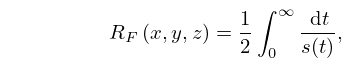
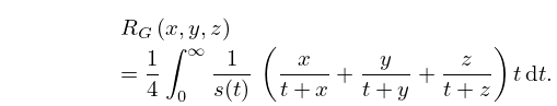
7: 19.16 Definitions

… ►

19.16.1 $$R_F(x,y,z)=\frac{1}{2}{\int }_0^{\mathrm{\infty }}\frac{dt}{s(t)},$$

ⓘ

Defines:

$R_F(x,y,z)$: symmetric elliptic integral of first kind

Symbols:

$dx$: differential of $x$ , $\int$: integral and $s(t)$: scaling factor

Referenced by:

§19.16(i), §19.16(i), §19.18(i), (19.25.35), (19.25.40), §19.25(vi)

Permalink:

http://dlmf.nist.gov/19.16.E1

Encodings:

pMML, png, TeX

See also:

Annotations for §19.16(i), §19.16 and Ch.19

►

19.16.2 $$R_J(x,y,z,p)=\frac{3}{2}{\int }_0^{\mathrm{\infty }}\frac{dt}{s(t)(t+p)},$$

ⓘ

Defines:

$R_J(x,y,z,p)$: symmetric elliptic integral of third kind

Symbols:

$dx$: differential of $x$ , $\int$: integral and $s(t)$: scaling factor

Referenced by:

§19.16(i), §19.19, §19.20(iii), §19.28

Permalink:

http://dlmf.nist.gov/19.16.E2

Encodings:

pMML, png, TeX

See also:

Annotations for §19.16(i), §19.16 and Ch.19

►

19.16.2_5 $$R_G(x,y,z)=\frac{1}{4}{\int }_0^{\mathrm{\infty }}\frac{1}{s(t)}\left(\frac{x}{t+x}+\frac{y}{t+y}+\frac{z}{t+z}\right)tdt.$$

ⓘ

Defines:

$R_G(x,y,z)$: symmetric elliptic integral of second kind

Symbols:

$dx$: differential of $x$ , $\int$: integral and $s(t)$: scaling factor

Source:

Carlson (1977b, (9.1-9))

Referenced by:

§19.16(i), §19.16(i), §19.21(ii), (19.23.7), (19.23.7), §19.23, Erratum (V1.1.0) for Rearrangement

Permalink:

http://dlmf.nist.gov/19.16.E2_5

Encodings:

pMML, png, TeX

Rearrangement (effective with 1.1.0):

This integral representation was moved from (19.23.7) and is taken as the definition of $R_G(x,y,z)$. We have also employed the notation $s(t)$ for the factor of radicals.

See also:

Annotations for §19.16(i), §19.16 and Ch.19

… ►

19.16.4 $$s(t)=\sqrt{t+x}\sqrt{t+y}\sqrt{t+z}.$$

ⓘ

Defines:

$s(t)$: scaling factor (locally)

Referenced by:

§19.16(i), (19.25.35), §19.25(vi)

Permalink:

http://dlmf.nist.gov/19.16.E4

Encodings:

pMML, png, TeX

See also:

Annotations for §19.16(i), §19.16 and Ch.19

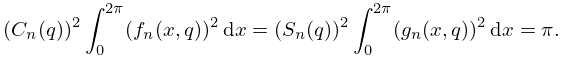
… ►It should be noted that the integrals (19.16.1)–(19.16.2_5) have been normalized so that $R_F(1,1,1)=R_J(1,1,1,1)=R_G(1,1,1)=1$. …

8: 18.2 General Orthogonal Polynomials

… ►The orthogonality relations (18.2.1)–(18.2.3) each determine the polynomials $p_n(x)$ uniquely up to constant factors, which may be fixed by suitable standardizations. … ►If the polynomials $p_n(x)$ ($n=0,1,\mathrm{\dots },N$) are orthogonal on a finite set $X$ of $N+1$ distinct points as in (18.2.3), then the polynomial $p_{N+1}(x)$ of degree $N+1$, up to a constant factor defined by (18.2.8) or (18.2.10), vanishes on $X$. … ►, of the form $w(x)dx$) nor is it necessarily unique, up to a positive constant factor. However, if OP’s have an orthogonality relation on a bounded interval, then their orthogonality measure is unique, up to a positive constant factor. …

9: 28.12 Definitions and Basic Properties

… ►In consequence, for the Floquet solutions $w(z)$ the factor ${\mathrm{e}}^{\pi \mathrm{i}\nu }$ in (28.2.14) is no longer $\pm 1$. … ►

28.12.2 $${\lambda }_{\nu }\left(-q\right)={\lambda }_{\nu }\left(q\right)={\lambda }_{-\nu }\left(q\right).$$

ⓘ

Symbols:

${\lambda }_{\nu +2n}\left(q\right)$: eigenvalues of Mathieu equation, $q=h^2$: parameter and $\nu$: complex parameter

Permalink:

http://dlmf.nist.gov/28.12.E2

Encodings:

pMML, png, TeX

See also:

Annotations for §28.12(i), §28.12 and Ch.28

►As in §28.7 values of $q$ for which (28.2.16) has simple roots $\lambda$ are called normal values with respect to $\nu$. For real values of $\nu$ and $q$ all the ${\lambda }_{\nu }\left(q\right)$ are real, and $q$ is normal. … ►If $q$ is a normal value of the corresponding equation (28.2.16), then these functions are uniquely determined as analytic functions of $z$ and $q$ by the normalization …

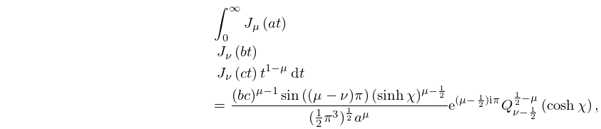
10: 10.22 Integrals

… ►

10.22.72 $${\int }_0^{\mathrm{\infty }}{J}_{\mu }\left(at\right)J_{\nu }\left(bt\right)J_{\nu }\left(ct\right)t^{1-\mu }dt=\frac{{(bc)}^{\mu -1}\sin \left((\mu -\nu )\pi \right){(\sinh \chi )}^{\mu -\frac{1}{2}}}{{(\frac{1}{2}{\pi }^3)}^{\frac{1}{2}}{a}^{\mu }}{\mathrm{e}}^{(\mu -\frac{1}{2})\mathrm{i}\pi }{Q}_{\nu -\frac{1}{2}}^{\frac{1}{2}-\mu }\left(\cosh \chi \right),$$ $\mathrm{\Re }\mu >-\frac{1}{2},\mathrm{\Re }\nu >-1,a>b+c,\cosh \chi =(a^2-b^2-c^2)/(2bc)$.

ⓘ

Symbols:

$J_{\nu }\left(z\right)$: Bessel function of the first kind, $Q_{\nu }^{\mu }\left(z\right)$: associated Legendre function of the second kind, $\pi$: the ratio of the circumference of a circle to its diameter, $\cos z$: cosine function, $dx$: differential of $x$ , $\mathrm{e}$: base of natural logarithm, $\cosh z$: hyperbolic cosine function, $\sinh z$: hyperbolic sine function, $\mathrm{i}$: imaginary unit, $\int$: integral, $\mathrm{\Re }$: real part, $\sin z$: sine function and $\nu$: complex parameter

Keywords:

Mellin transform

Referenced by:

§10.22(iv), §10.22(iv), Erratum (V1.0.21) for Equation (10.22.72)

Permalink:

http://dlmf.nist.gov/10.22.E72

Encodings:

pMML, png, TeX

Clarification (effective with 1.0.21):

Originally, the factor on the right-hand side was written as $\frac{{(bc)}^{\mu -1}\cos \left(\nu \pi \right){(\sinh \chi )}^{\mu -\frac{1}{2}}}{{(\frac{1}{2}{\pi }^3)}^{\frac{1}{2}}{a}^{\mu }}$, which was taken directly from Watson (1944, p. 412, (13.46.5)), who uses a different normalization for the associated Legendre functions of the second kind $Q_{\nu }^{\mu }$. Watson’s $Q_{\nu }^{\mu }$ equals $\frac{\sin \left((\nu +\mu )\pi \right)}{\sin \left(\nu \pi \right)}{\mathrm{e}}^{-\mu \pi \mathrm{i}}{Q}_{\nu }^{\mu }$ in the DLMF.

See also:

Annotations for §10.22(iv), §10.22(iv), §10.22 and Ch.10

…