stable regions

SearchAdvancedHelp

(0.002 seconds)

6 matching pages

1: 28.17 Stability as $x\to \pm \mathrm{\infty }$

§28.17 Stability as $x\to \pm \mathrm{\infty }$

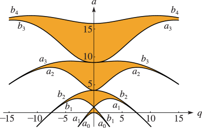
… ►For real $a$ and $q$ $(\ne 0)$ the stable regions are the open regions indicated in color in Figure 28.17.1. … ►

►►

Figure 28.17.1: Stability chart for eigenvalues of Mathieu’s equation (28.2.1). Magnify

2: 9.17 Methods of Computation

… ►In the case of the Scorer functions, integration of the differential equation (9.12.1) is more difficult than (9.2.1), because in some regions stable directions of integration do not exist. …

3: 28.33 Physical Applications

… ►Hence from §28.17 the corresponding Mathieu equation is stable or unstable according as $(q,a)$ is in the intersection of $ℒ$ with the colored or the uncolored open regions depicted in Figure 28.17.1. …

4: 33.23 Methods of Computation

… ►When numerical values of the Coulomb functions are available for some radii, their values for other radii may be obtained by direct numerical integration of equations (33.2.1) or (33.14.1), provided that the integration is carried out in a stable direction (§3.7). … ►In a similar manner to §33.23(iii) the recurrence relations of §§33.4 or 33.17 can be used for a range of values of the integer $\mathrm{\ell }$, provided that the recurrence is carried out in a stable direction (§3.6). … ►Bardin et al. (1972) describes ten different methods for the calculation of $F_{\mathrm{\ell }}$ and $G_{\mathrm{\ell }}$, valid in different regions of the ($\eta ,\rho$)-plane. … ►Hull and Breit (1959) and Barnett (1981b) give WKBJ approximations for $F_0$ and $G_0$ in the region inside the turning point: .

5: 18.40 Methods of Computation

… ►A simple set of choices is spelled out in Gordon (1968) which gives a numerically stable algorithm for direct computation of the recursion coefficients in terms of the moments, followed by construction of the J-matrix and quadrature weights and abscissas, and we will follow this approach: Let $N$ be a positive integer and define …See Gautschi (1983) for examples of numerically stable and unstable use of the above recursion relations, and how one can then usefully differentiate between numerical results of low and high precision, as produced thereby. … ►The question is then: how is this possible given only $F_N(z)$, rather than $F(z)$ itself? $F_N(z)$ often converges to smooth results for $z$ off the real axis for $\mathrm{\Im }z$ at a distance greater than the pole spacing of the $x_n$, this may then be followed by approximate numerical analytic continuation via fitting to lower order continued fractions (either Padé, see §3.11(iv), or pointwise continued fraction approximants, see Schlessinger (1968, Appendix)), to $F_N(z)$ and evaluating these on the real axis in regions of higher pole density that those of the approximating function. … ►

►►

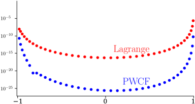
Figure 18.40.2: Derivative Rule inversions for $w^{\mathrm{RCP}}(x)$ carried out via Lagrange and PWCF interpolations. …For the derivative rule Lagrange interpolation (red points) gives $\sim 15$ digits in the central region, while PWCF interpolation (blue points) gives $\sim 25$. Magnify

…

6: 3.10 Continued Fractions

… ►For example, by converting the Maclaurin expansion of $\arctan z$ (4.24.3), we obtain a continued fraction with the same region of convergence ($\left|z\right|\le 1$, $z\ne \pm \mathrm{i}$), whereas the continued fraction (4.25.4) converges for all $z\in ℂ$ except on the branch cuts from $\mathrm{i}$ to $\mathrm{i}\mathrm{\infty }$ and $-\mathrm{i}$ to $-\mathrm{i}\mathrm{\infty }$. … ►A more stable version of the algorithm is discussed in Stokes (1980). … ►In general this algorithm is more stable than the forward algorithm; see Jones and Thron (1974). …