limiting form as a Bessel function

SearchAdvancedHelp

(0.011 seconds)

11—20 of 31 matching pages

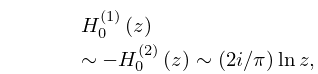
11: 10.7 Limiting Forms

§10.7 Limiting Forms

… ►

10.7.2 $$H_0^{(1)}\left(z\right)\sim -H_0^{(2)}\left(z\right)\sim (2\mathrm{i}/\pi )\ln z,$$

ⓘ

Symbols:

$H_{\nu }^{(1)}\left(z\right)$: Bessel function of the third kind (or Hankel function), $H_{\nu }^{(2)}\left(z\right)$: Bessel function of the third kind (or Hankel function), $\sim$: asymptotic equality, $\pi$: the ratio of the circumference of a circle to its diameter, $\mathrm{i}$: imaginary unit, $\ln z$: principal branch of logarithm function and $z$: complex variable

A&S Ref:

9.1.8

Referenced by:

§10.7(i)

Permalink:

http://dlmf.nist.gov/10.7.E2

Encodings:

pMML, png, TeX

See also:

Annotations for §10.7(i), §10.7 and Ch.10

… ►For $H_{-\nu }^{(1)}\left(z\right)$ and $H_{-\nu }^{(2)}\left(z\right)$ when $\mathrm{\Re }\nu >0$ combine (10.4.6) and (10.7.7). For $H_{\mathrm{i}\nu }^{(1)}\left(z\right)$ and $H_{\mathrm{i}\nu }^{(2)}\left(z\right)$ when $\nu \in ℝ$ and $\nu \ne 0$ combine (10.4.3), (10.7.3), and (10.7.6). … ►For the corresponding results for $H_{\nu }^{(1)}\left(z\right)$ and $H_{\nu }^{(2)}\left(z\right)$ see (10.2.5) and (10.2.6).

12: 10.25 Definitions

… ►

§10.25(i) Modified Bessel’s Equation

… ►Its solutions are called modified Bessel functions or Bessel functions of imaginary argument. ►

§10.25(ii) Standard Solutions

… ►

Branch Conventions

…

13: 11.9 Lommel Functions

§11.9 Lommel Functions

… ►The inhomogeneous Bessel differential equation … ►the right-hand side being replaced by its limiting form when $\mu \pm \nu$ is an odd negative integer. … ►

§11.9(ii) Expansions in Series of Bessel Functions

… ► …

14: Mathematical Introduction

… ►The mathematical content of the NIST Handbook of Mathematical Functions has been produced over a ten-year period. … ►This is because $𝐅$ is akin to the notation used for Bessel functions (§10.2(ii)), inasmuch as $𝐅$ is an entire function of each of its parameters $a$, $b$, and $c$:​ this results in fewer restrictions and simpler equations. … ►Other examples are: (a) the notation for the Ferrers functions—also known as associated Legendre functions on the cut—for which existing notations can easily be confused with those for other associated Legendre functions (§14.1); (b) the spherical Bessel functions for which existing notations are unsymmetric and inelegant (§§10.47(i) and 10.47(ii)); and (c) elliptic integrals for which both Legendre’s forms and the more recent symmetric forms are treated fully (Chapter 19). … ►Special functions with a complex variable are depicted as colored 3D surfaces in a similar way to functions of two real variables, but with the vertical height corresponding to the modulus (absolute value) of the function. … ►For equations or other technical information that appeared previously in AMS 55, the DLMF usually includes the corresponding AMS 55 equation number, or other form of reference, together with corrections, if needed. …

15: 10.50 Wronskians and Cross-Products

§10.50 Wronskians and Cross-Products

… ►

$$𝒲\left\{{𝗁}_n^{(1)}\left(z\right),{𝗁}_n^{(2)}\left(z\right)\right\}=-2\mathrm{i}{z}^{-2}.$$

… ►

10.50.4 $${𝗃}_0\left(z\right){𝗃}_n\left(z\right)+{𝗒}_0\left(z\right){𝗒}_n\left(z\right)=\cos \left(\frac{1}{2}n\pi \right)\sum _{k=0}^{\lfloor n/2\rfloor }{(-1)}^k\frac{a_{2k}(n+\frac{1}{2})}{z^{2k+2}}+\sin \left(\frac{1}{2}n\pi \right)\sum _{k=0}^{\lfloor (n-1)/2\rfloor }{(-1)}^k\frac{a_{2k+1}(n+\frac{1}{2})}{z^{2k+3}},$$

ⓘ

Symbols:

$\pi$: the ratio of the circumference of a circle to its diameter, $\cos z$: cosine function, $\lfloor x\rfloor$: floor of $x$ , $\sin z$: sine function, ${𝗃}_n\left(z\right)$: spherical Bessel function of the first kind, ${𝗒}_n\left(z\right)$: spherical Bessel function of the second kind, $n$: integer, $k$: nonnegative integer, $z$: complex variable and $a_k(\nu )$: polynomial coefficient

A&S Ref:

10.1.33 (modified)

Referenced by:

§10.50, §10.50

Permalink:

http://dlmf.nist.gov/10.50.E4

Encodings:

pMML, png, TeX

See also:

Annotations for §10.50 and Ch.10

►where $a_k(n+\frac{1}{2})$ is given by (10.49.1). ►Results corresponding to (10.50.3) and (10.50.4) for ${𝗂}_n^{(1)}\left(z\right)$ and ${𝗂}_n^{(2)}\left(z\right)$ are obtainable via (10.47.12).

16: 11.13 Methods of Computation

… ►

§11.13(i) Introduction

►Subsequent subsections treat the computation of Struve functions. The treatment of Lommel and Anger–Weber functions is similar. … ►Although the power-series expansions (11.2.1) and (11.2.2), and the Bessel-function expansions of §11.4(iv) converge for all finite values of $z$, they are cumbersome to use when $|z|$ is large owing to slowness of convergence and cancellation. … ►Then from the limiting forms for small argument (§§11.2(i), 10.7(i), 10.30(i)), limiting forms for large argument (§§11.6(i), 10.7(ii), 10.30(ii)), and the connection formulas (11.2.5) and (11.2.6), it is seen that ${𝐇}_{\nu }\left(x\right)$ and ${𝐋}_{\nu }\left(x\right)$ can be computed in a stable manner by integrating forwards, that is, from the origin toward infinity. …

17: 1.18 Linear Second Order Differential Operators and Eigenfunction Expansions

… ►The eigenfunctions form a complete orthogonal basis in $L^2\left(X\right)$, and we can take the basis as orthonormal: … ►Let $T$ be the self adjoint extension of a formally self-adjoint differential operator $ℒ$ of the form (1.18.28) on an unbounded interval $X\subset ℝ$, which we will take as $X=[0,+\mathrm{\infty })$, and assume that $q(x)\to 0$ monotonically as $x\to \mathrm{\infty }$, and that the eigenfunctions are non-vanishing but bounded in this same limit. … ►By Bessel’s differential equation in the form (10.13.1) we have the functions $\sqrt{x}{J}_{\nu }\left(x\sqrt{\lambda }\right)$ ($\lambda \ge 0$, for $J_{\nu }$ see §10.2(ii)) as eigenfunctions with eigenvalue $\lambda$ of the self-adjoint extension of the differential operator … ►In general, operators $T$ being formally self-adjoint second order differential operators of the form (1.18.28), with $X$ unbounded, will have both a continuous and a point spectrum, and thus, correspondingly, $non-L^2\left(X\right)$ eigenfunctions as in §1.18(vi) and $L^2\left(X\right)$ eigenfunctions as in §1.18(v). … ► A boundary value for the end point $a$ is a linear form $ℬ$ on $𝒟({ℒ}^{\ast })$ of the form …

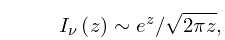
18: 10.30 Limiting Forms

§10.30 Limiting Forms

►

§10.30(i) $z\to 0$

… ►For $K_{\nu }\left(x\right)$, when $\nu$ is purely imaginary and $x\to 0+$, see (10.45.2) and (10.45.7). … ►

10.30.4 $$I_{\nu }\left(z\right)\sim {\mathrm{e}}^z/\sqrt{2\pi z},$$ $|\mathrm{ph}z|\le \frac{1}{2}\pi -\delta$,

ⓘ

Symbols:

$\sim$: asymptotic equality, $\pi$: the ratio of the circumference of a circle to its diameter, $\mathrm{e}$: base of natural logarithm, $I_{\nu }\left(z\right)$: modified Bessel function of the first kind, $\mathrm{ph}$: phase, $z$: complex variable, $\nu$: complex parameter and $\delta$: small positive constant

Permalink:

http://dlmf.nist.gov/10.30.E4

Encodings:

pMML, png, TeX

See also:

Annotations for §10.30(ii), §10.30 and Ch.10

… ►For $K_{\nu }\left(z\right)$ see (10.25.3).

19: 33.5 Limiting Forms for Small $\rho$, Small $|\eta |$, or Large $\mathrm{\ell }$

§33.5 Limiting Forms for Small $\rho$, Small $|\eta |$, or Large $\mathrm{\ell }$

►

§33.5(i) Small $\rho$

… ►For the functions $𝗃$, $𝗒$, $J$, $Y$ see §§10.47(ii), 10.2(ii). … ►

§33.5(iii) Small $|\eta |$

… ►

§33.5(iv) Large $\mathrm{\ell }$

…

20: 10.72 Mathematical Applications

… ►Bessel functions and modified Bessel functions are often used as approximants in the construction of uniform asymptotic approximations and expansions for solutions of linear second-order differential equations containing a parameter. … ►If $f(z)$ has a double zero $z_0$, or more generally $z_0$ is a zero of order $m$, $m=2,3,4,\mathrm{\dots }$, then uniform asymptotic approximations (but not expansions) can be constructed in terms of Bessel functions, or modified Bessel functions, of order $1/(m+2)$. …The order of the approximating Bessel functions, or modified Bessel functions, is $1/(\lambda +2)$, except in the case when $g(z)$ has a double pole at $z_0$. … ►In regions in which the function $f(z)$ has a simple pole at $z=z_0$ and ${(z-z_0)}^{2}g(z)$ is analytic at $z=z_0$ (the case $\lambda =-1$ in §10.72(i)), asymptotic expansions of the solutions $w$ of (10.72.1) for large $u$ can be constructed in terms of Bessel functions and modified Bessel functions of order $\pm \sqrt{1+4\rho }$, where $\rho$ is the limiting value of ${(z-z_0)}^{2}g(z)$ as $z\to z_0$. … ►