lattice walks

SearchAdvancedHelp

(0.002 seconds)

11—20 of 59 matching pages

11: 23.23 Tables

… ►2 in Abramowitz and Stegun (1964) gives values of $\mathrm{\wp }\left(z\right)$, ${\mathrm{\wp }}^{\prime }\left(z\right)$, and $\zeta \left(z\right)$ to 7 or 8D in the rectangular and rhombic cases, normalized so that ${\omega }_1=1$ and ${\omega }_3=\mathrm{i}a$ (rectangular case), or ${\omega }_1=1$ and ${\omega }_3=\frac{1}{2}+\mathrm{i}a$ (rhombic case), for $a$ = 1. …05, and in the case of $\mathrm{\wp }\left(z\right)$ the user may deduce values for complex $z$ by application of the addition theorem (23.10.1). ►Abramowitz and Stegun (1964) also includes other tables to assist the computation of the Weierstrass functions, for example, the generators as functions of the lattice invariants $g_2$ and $g_3$. …

12: 23.6 Relations to Other Functions

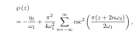
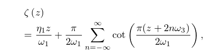
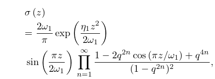
… ►In this subsection $2{\omega }_1$, $2{\omega }_3$ are any pair of generators of the lattice $𝕃$, and the lattice roots $e_1$, $e_2$, $e_3$ are given by (23.3.9). … ►For further results for the $\sigma$-function see Lawden (1989, §6.2). … ►Again, in Equations (23.6.16)–(23.6.26), $2{\omega }_1,2{\omega }_3$ are any pair of generators of the lattice $𝕃$ and $e_1,e_2,e_3$ are given by (23.3.9). … ►

Rectangular Lattice

… ►

General Lattice

…

13: 23.19 Interrelations

… ►

23.19.3 $$J\left(\tau \right)=\frac{g_2^3}{g_2^3-27g_3^2},$$

ⓘ

Symbols:

$J\left(\tau \right)$: Klein’s complete invariant, $g_j$: Weierstrass lattice invariants $g_2$, $g_3$ , $𝕃$: lattice and $\tau$: complex variable

Permalink:

http://dlmf.nist.gov/23.19.E3

Encodings:

pMML, png, TeX

See also:

Annotations for §23.19 and Ch.23

►where $g_2,g_3$ are the invariants of the lattice $𝕃$ with generators $1$ and $\tau$; see §23.3(i). …

14: 23.1 Special Notation

… ► ►►►►

$𝕃$	lattice in $ℂ$.
…
$2{\omega }_1,2{\omega }_3$	lattice generators ($\mathrm{\Im }\left({\omega }_3/{\omega }_1\right)>0$).
…
$\mathrm{\Delta }$	discriminant $g_2^3-27g_3^2$.
…

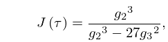
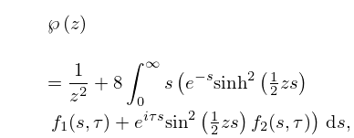
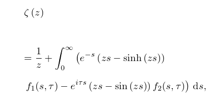
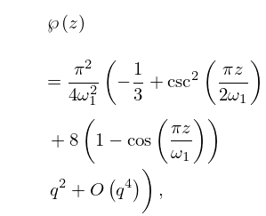
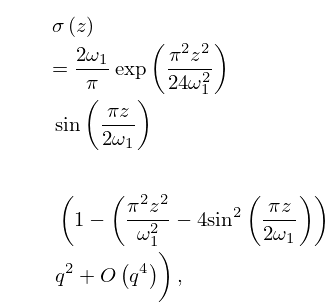
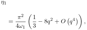
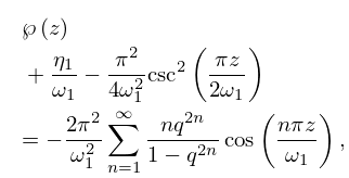
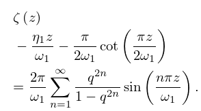
►The main functions treated in this chapter are the Weierstrass $\mathrm{\wp }$-function $\mathrm{\wp }\left(z\right)=\mathrm{\wp }\left(z|𝕃\right)=\mathrm{\wp }(z;g_2,g_3)$; the Weierstrass zeta function $\zeta \left(z\right)=\zeta \left(z|𝕃\right)=\zeta (z;g_2,g_3)$; the Weierstrass sigma function $\sigma \left(z\right)=\sigma \left(z|𝕃\right)=\sigma (z;g_2,g_3)$; the elliptic modular function $\lambda \left(\tau \right)$; Klein’s complete invariant $J\left(\tau \right)$; Dedekind’s eta function $\eta \left(\tau \right)$. … ►Abramowitz and Stegun (1964, Chapter 18) considers only rectangular and rhombic lattices (§23.5); ${\omega }_1$, ${\omega }_3$ are replaced by $\omega$, ${\omega }^{\prime }$ for the former and by ${\omega }_2$, ${\omega }^{\prime }$ for the latter. …

15: 23.13 Zeros

… ►For information on the zeros of $\mathrm{\wp }\left(z\right)$ see Eichler and Zagier (1982).

16: 23.11 Integral Representations

… ►

23.11.2 $$\mathrm{\wp }\left(z\right)=\frac{1}{z^2}+8{\int }_0^{\mathrm{\infty }}s\left({\mathrm{e}}^{-s}{\sinh }^2\left(\frac{1}{2}zs\right)f_1(s,\tau )+{\mathrm{e}}^{\mathrm{i}\tau s}{\sin }^2\left(\frac{1}{2}zs\right)f_2(s,\tau )\right)ds,$$

ⓘ

Symbols:

$\mathrm{\wp }\left(z\right)$ (= $\mathrm{\wp }\left(z|𝕃\right)$ = $\mathrm{\wp }(z;g_2,g_3)$): Weierstrass $\mathrm{\wp }$-function, $dx$: differential of $x$ , $\mathrm{e}$: base of natural logarithm, $\sinh z$: hyperbolic sine function, $\mathrm{i}$: imaginary unit, $\int$: integral, $\sin z$: sine function, $𝕃$: lattice, $z$: complex, $\tau$: complex variable and $f_j(s,\tau )$: functions

Permalink:

http://dlmf.nist.gov/23.11.E2

Encodings:

pMML, png, TeX

See also:

Annotations for §23.11 and Ch.23

… ►

23.11.3 $$\zeta \left(z\right)=\frac{1}{z}+{\int }_0^{\mathrm{\infty }}\left({\mathrm{e}}^{-s}\left(zs-\sinh \left(zs\right)\right)f_1(s,\tau )-{\mathrm{e}}^{\mathrm{i}\tau s}\left(zs-\sin \left(zs\right)\right)f_2(s,\tau )\right)ds,$$

ⓘ

Symbols:

$\zeta \left(z\right)$ (= $\zeta \left(z|𝕃\right)$ = $\zeta (z;g_2,g_3)$): Weierstrass zeta function, $dx$: differential of $x$ , $\mathrm{e}$: base of natural logarithm, $\sinh z$: hyperbolic sine function, $\mathrm{i}$: imaginary unit, $\int$: integral, $\sin z$: sine function, $𝕃$: lattice, $z$: complex, $\tau$: complex variable and $f_j(s,\tau )$: functions

Permalink:

http://dlmf.nist.gov/23.11.E3

Encodings:

pMML, png, TeX

See also:

Annotations for §23.11 and Ch.23

…

17: 23.12 Asymptotic Approximations

… ►

23.12.1 $$\mathrm{\wp }\left(z\right)=\frac{{\pi }^2}{4{\omega }_1^2}\left(-\frac{1}{3}+{\csc }^2\left(\frac{\pi z}{2{\omega }_1}\right)+8\left(1-\cos \left(\frac{\pi z}{{\omega }_1}\right)\right)q^2+O\left(q^4\right)\right),$$

ⓘ

Symbols:

$O\left(x\right)$: order not exceeding, $\mathrm{\wp }\left(z\right)$ (= $\mathrm{\wp }\left(z|𝕃\right)$ = $\mathrm{\wp }(z;g_2,g_3)$): Weierstrass $\mathrm{\wp }$-function, $\pi$: the ratio of the circumference of a circle to its diameter, $\csc z$: cosecant function, $\cos z$: cosine function, $𝕃$: lattice, $q$: nome, $z$: complex and ${\omega }_1$, ${\omega }_3$, ${\omega }_2=-{\omega }_1-{\omega }_3$: lattice generators

Referenced by:

§23.12

Permalink:

http://dlmf.nist.gov/23.12.E1

Encodings:

pMML, png, TeX

See also:

Annotations for §23.12 and Ch.23

►

23.12.2 $$\zeta \left(z\right)=\frac{{\pi }^2}{4{\omega }_1^2}\left(\frac{z}{3}+\frac{2{\omega }_1}{\pi }\cot \left(\frac{\pi z}{2{\omega }_1}\right)-8\left(z-\frac{{\omega }_1}{\pi }\sin \left(\frac{\pi z}{{\omega }_1}\right)\right)q^2+O\left(q^4\right)\right),$$

ⓘ

Symbols:

$O\left(x\right)$: order not exceeding, $\zeta \left(z\right)$ (= $\zeta \left(z|𝕃\right)$ = $\zeta (z;g_2,g_3)$): Weierstrass zeta function, $\pi$: the ratio of the circumference of a circle to its diameter, $\cot z$: cotangent function, $\sin z$: sine function, $𝕃$: lattice, $q$: nome, $z$: complex and ${\omega }_1$, ${\omega }_3$, ${\omega }_2=-{\omega }_1-{\omega }_3$: lattice generators

Referenced by:

§23.12, Erratum (V1.0.23) for Equation (23.12.2)

Permalink:

http://dlmf.nist.gov/23.12.E2

Encodings:

pMML, png, TeX

Correction (effective with 1.0.23):

The factor of 2, previously omitted from the denominator of the argument of the $\cot$ function has been inserted.

Suggested 2019-05-27 by Blagoje Oblak

See also:

Annotations for §23.12 and Ch.23

►

23.12.3 $$\sigma \left(z\right)=\frac{2{\omega }_1}{\pi }\exp \left(\frac{{\pi }^2{z}^2}{24{\omega }_1^2}\right)\sin \left(\frac{\pi z}{2{\omega }_1}\right)\left(1-\left(\frac{{\pi }^2{z}^2}{{\omega }_1^2}-4{\sin }^2\left(\frac{\pi z}{2{\omega }_1}\right)\right)q^2+O\left(q^4\right)\right),$$

ⓘ

Symbols:

$O\left(x\right)$: order not exceeding, $\sigma \left(z\right)$ (= $\sigma \left(z|𝕃\right)$ = $\sigma (z;g_2,g_3)$): Weierstrass sigma function, $\pi$: the ratio of the circumference of a circle to its diameter, $\exp z$: exponential function, $\sin z$: sine function, $𝕃$: lattice, $q$: nome, $z$: complex and ${\omega }_1$, ${\omega }_3$, ${\omega }_2=-{\omega }_1-{\omega }_3$: lattice generators

Permalink:

http://dlmf.nist.gov/23.12.E3

Encodings:

pMML, png, TeX

See also:

Annotations for §23.12 and Ch.23

… ►

23.12.4 $${\eta }_1=\frac{{\pi }^2}{4{\omega }_1}\left(\frac{1}{3}-8q^2+O\left(q^4\right)\right),$$

ⓘ

Symbols:

$O\left(x\right)$: order not exceeding, $\pi$: the ratio of the circumference of a circle to its diameter, $q$: nome, ${\omega }_1$, ${\omega }_3$, ${\omega }_2=-{\omega }_1-{\omega }_3$: lattice generators and ${\eta }_j$: complex number

Referenced by:

§23.12

Permalink:

http://dlmf.nist.gov/23.12.E4

Encodings:

pMML, png, TeX

See also:

Annotations for §23.12 and Ch.23

…

18: 31.2 Differential Equations

… ►

$k^2=(e_2-e_3)/(e_1-e_3),$

… ►

$e_1=\mathrm{\wp }\left({\omega }_1\right),$

►

$e_2=\mathrm{\wp }\left({\omega }_2\right),$

… ►

$e_1+e_2+e_3=0,$

►where $2{\omega }_1$ and $2{\omega }_3$ with $\mathrm{\Im }\left({\omega }_3/{\omega }_1\right)>0$ are generators of the lattice $𝕃$ for $\mathrm{\wp }\left(z|𝕃\right)$. …

19: 23.8 Trigonometric Series and Products

… ►

23.8.1 $$\mathrm{\wp }\left(z\right)+\frac{{\eta }_1}{{\omega }_1}-\frac{{\pi }^2}{4{\omega }_1^2}{\csc }^2\left(\frac{\pi z}{2{\omega }_1}\right)=-\frac{2{\pi }^2}{{\omega }_1^2}\sum _{n=1}^{\mathrm{\infty }}\frac{n{q}^{2n}}{1-q^{2n}}\cos \left(\frac{n\pi z}{{\omega }_1}\right),$$

ⓘ

Symbols:

$\mathrm{\wp }\left(z\right)$ (= $\mathrm{\wp }\left(z|𝕃\right)$ = $\mathrm{\wp }(z;g_2,g_3)$): Weierstrass $\mathrm{\wp }$-function, $\pi$: the ratio of the circumference of a circle to its diameter, $\csc z$: cosecant function, $\cos z$: cosine function, $𝕃$: lattice, $q$: nome, $n$: integer, $z$: complex, ${\omega }_1$, ${\omega }_3$, ${\omega }_2=-{\omega }_1-{\omega }_3$: lattice generators and ${\eta }_j$: complex number

Permalink:

http://dlmf.nist.gov/23.8.E1

Encodings:

pMML, png, TeX

See also:

Annotations for §23.8(i), §23.8 and Ch.23

►

23.8.2 $$\zeta \left(z\right)-\frac{{\eta }_{1}z}{{\omega }_1}-\frac{\pi }{2{\omega }_1}\cot \left(\frac{\pi z}{2{\omega }_1}\right)=\frac{2\pi }{{\omega }_1}\sum _{n=1}^{\mathrm{\infty }}\frac{q^{2n}}{1-q^{2n}}\sin \left(\frac{n\pi z}{{\omega }_1}\right).$$

ⓘ

Symbols:

$\zeta \left(z\right)$ (= $\zeta \left(z|𝕃\right)$ = $\zeta (z;g_2,g_3)$): Weierstrass zeta function, $\pi$: the ratio of the circumference of a circle to its diameter, $\cot z$: cotangent function, $\sin z$: sine function, $𝕃$: lattice, $q$: nome, $n$: integer, $z$: complex, ${\omega }_1$, ${\omega }_3$, ${\omega }_2=-{\omega }_1-{\omega }_3$: lattice generators and ${\eta }_j$: complex number

Permalink:

http://dlmf.nist.gov/23.8.E2

Encodings:

pMML, png, TeX

See also:

Annotations for §23.8(i), §23.8 and Ch.23

… ►

23.8.3 $$\mathrm{\wp }\left(z\right)=-\frac{{\eta }_1}{{\omega }_1}+\frac{{\pi }^2}{4{\omega }_1^2}\sum _{n=-\mathrm{\infty }}^{\mathrm{\infty }}{\csc }^2\left(\frac{\pi (z+2n{\omega }_3)}{2{\omega }_1}\right),$$

ⓘ

Symbols:

$\mathrm{\wp }\left(z\right)$ (= $\mathrm{\wp }\left(z|𝕃\right)$ = $\mathrm{\wp }(z;g_2,g_3)$): Weierstrass $\mathrm{\wp }$-function, $\pi$: the ratio of the circumference of a circle to its diameter, $\csc z$: cosecant function, $𝕃$: lattice, $n$: integer, $z$: complex, ${\omega }_1$, ${\omega }_3$, ${\omega }_2=-{\omega }_1-{\omega }_3$: lattice generators and ${\eta }_j$: complex number

Permalink:

http://dlmf.nist.gov/23.8.E3

Encodings:

pMML, png, TeX

See also:

Annotations for §23.8(ii), §23.8 and Ch.23

►

23.8.4 $$\zeta \left(z\right)=\frac{{\eta }_{1}z}{{\omega }_1}+\frac{\pi }{2{\omega }_1}\sum _{n=-\mathrm{\infty }}^{\mathrm{\infty }}\cot \left(\frac{\pi (z+2n{\omega }_3)}{2{\omega }_1}\right),$$

ⓘ

Symbols:

$\zeta \left(z\right)$ (= $\zeta \left(z|𝕃\right)$ = $\zeta (z;g_2,g_3)$): Weierstrass zeta function, $\pi$: the ratio of the circumference of a circle to its diameter, $\cot z$: cotangent function, $𝕃$: lattice, $n$: integer, $z$: complex, ${\omega }_1$, ${\omega }_3$, ${\omega }_2=-{\omega }_1-{\omega }_3$: lattice generators and ${\eta }_j$: complex number

Referenced by:

§23.8(ii)

Permalink:

http://dlmf.nist.gov/23.8.E4

Encodings:

pMML, png, TeX

See also:

Annotations for §23.8(ii), §23.8 and Ch.23

… ►

23.8.6 $$\sigma \left(z\right)=\frac{2{\omega }_1}{\pi }\exp \left(\frac{{\eta }_1{z}^2}{2{\omega }_1}\right)\sin \left(\frac{\pi z}{2{\omega }_1}\right)\prod _{n=1}^{\mathrm{\infty }}\frac{1-2q^{2n}\cos \left(\pi z/{\omega }_1\right)+q^{4n}}{{(1-q^{2n})}^2},$$

ⓘ

Symbols:

$\sigma \left(z\right)$ (= $\sigma \left(z|𝕃\right)$ = $\sigma (z;g_2,g_3)$): Weierstrass sigma function, $\pi$: the ratio of the circumference of a circle to its diameter, $\cos z$: cosine function, $\exp z$: exponential function, $\sin z$: sine function, $𝕃$: lattice, $q$: nome, $n$: integer, $z$: complex, ${\omega }_1$, ${\omega }_3$, ${\omega }_2=-{\omega }_1-{\omega }_3$: lattice generators and ${\eta }_j$: complex number

Permalink:

http://dlmf.nist.gov/23.8.E6

Encodings:

pMML, png, TeX

See also:

Annotations for §23.8(iii), §23.8 and Ch.23

…

20: 26.2 Basic Definitions

… ►

Lattice Path

►A lattice path is a directed path on the plane integer lattice $\{0,1,2,\mathrm{\dots }\}\times \{0,1,2,\mathrm{\dots }\}$. …For an example see Figure 26.9.2. ►A k-dimensional lattice path is a directed path composed of segments that connect vertices in ${\{0,1,2,\mathrm{\dots }\}}^k$ so that each segment increases one coordinate by exactly one unit. …