lattice walks

SearchAdvancedHelp

(0.002 seconds)

1—10 of 59 matching pages

1: 16.24 Physical Applications

… ►

§16.24(i) Random Walks

►Generalized hypergeometric functions and Appell functions appear in the evaluation of the so-called Watson integrals which characterize the simplest possible lattice walks. They are also potentially useful for the solution of more complicated restricted lattice walk problems, and the 3D Ising model; see Barber and Ninham (1970, pp. 147–148). …

2: 23.7 Quarter Periods

… ►

23.7.1 $$\mathrm{\wp }\left(\frac{1}{2}{\omega }_1\right)=e_1+\sqrt{(e_1-e_3)(e_1-e_2)}=e_1+{\omega }_1^{-2}{(K\left(k\right))}^2{k}^{\prime },$$

ⓘ

Symbols:

$\mathrm{\wp }\left(z\right)$ (= $\mathrm{\wp }\left(z|𝕃\right)$ = $\mathrm{\wp }(z;g_2,g_3)$): Weierstrass $\mathrm{\wp }$-function, $e_j$: Weierstrass lattice roots, $K\left(k\right)$: Legendre’s complete elliptic integral of the first kind, $𝕃$: lattice, ${\omega }_1$, ${\omega }_3$, ${\omega }_2=-{\omega }_1-{\omega }_3$: lattice generators, $k$: modulus and $k^{\prime }$: complementary modulus

A&S Ref:

18.3.18

Permalink:

http://dlmf.nist.gov/23.7.E1

Encodings:

pMML, png, TeX

See also:

Annotations for §23.7 and Ch.23

►

23.7.2 $$\mathrm{\wp }\left(\frac{1}{2}{\omega }_2\right)=e_2-\mathrm{i}\sqrt{(e_1-e_2)(e_2-e_3)}=e_2-\mathrm{i}{\omega }_1^{-2}{(K\left(k\right))}^{2}k{k}^{\prime },$$

ⓘ

Symbols:

$\mathrm{\wp }\left(z\right)$ (= $\mathrm{\wp }\left(z|𝕃\right)$ = $\mathrm{\wp }(z;g_2,g_3)$): Weierstrass $\mathrm{\wp }$-function, $e_j$: Weierstrass lattice roots, $K\left(k\right)$: Legendre’s complete elliptic integral of the first kind, $\mathrm{i}$: imaginary unit, $𝕃$: lattice, ${\omega }_1$, ${\omega }_3$, ${\omega }_2=-{\omega }_1-{\omega }_3$: lattice generators, $k$: modulus and $k^{\prime }$: complementary modulus

A&S Ref:

18.3.18

Permalink:

http://dlmf.nist.gov/23.7.E2

Encodings:

pMML, png, TeX

See also:

Annotations for §23.7 and Ch.23

►

23.7.3 $$\mathrm{\wp }\left(\frac{1}{2}{\omega }_3\right)=e_3-\sqrt{(e_1-e_3)(e_2-e_3)}=e_3-{\omega }_1^{-2}{(K\left(k\right))}^{2}k,$$

ⓘ

Symbols:

$\mathrm{\wp }\left(z\right)$ (= $\mathrm{\wp }\left(z|𝕃\right)$ = $\mathrm{\wp }(z;g_2,g_3)$): Weierstrass $\mathrm{\wp }$-function, $e_j$: Weierstrass lattice roots, $K\left(k\right)$: Legendre’s complete elliptic integral of the first kind, $𝕃$: lattice, ${\omega }_1$, ${\omega }_3$, ${\omega }_2=-{\omega }_1-{\omega }_3$: lattice generators and $k$: modulus

A&S Ref:

18.3.18

Permalink:

http://dlmf.nist.gov/23.7.E3

Encodings:

pMML, png, TeX

See also:

Annotations for §23.7 and Ch.23

►where $k,k^{\prime }$ and the square roots are real and positive when the lattice is rectangular; otherwise they are determined by continuity from the rectangular case.

3: 23.3 Differential Equations

… ►The lattice invariants are defined by … ►The lattice roots satisfy the cubic equation …and are denoted by $e_1,e_2,e_3$. … ►Let $g_2^3\ne 27g_3^2$, or equivalently $\mathrm{\Delta }$ be nonzero, or $e_1,e_2,e_3$ be distinct. … ►Conversely, $g_2$, $g_3$, and the set $\{e_1,e_2,e_3\}$ are determined uniquely by the lattice $𝕃$ independently of the choice of generators. …

4: 23.14 Integrals

… ►

23.14.1 $$\int \mathrm{\wp }\left(z\right)dz=-\zeta \left(z\right),$$

ⓘ

Symbols:

$\mathrm{\wp }\left(z\right)$ (= $\mathrm{\wp }\left(z|𝕃\right)$ = $\mathrm{\wp }(z;g_2,g_3)$): Weierstrass $\mathrm{\wp }$-function, $\zeta \left(z\right)$ (= $\zeta \left(z|𝕃\right)$ = $\zeta (z;g_2,g_3)$): Weierstrass zeta function, $dx$: differential of $x$ , $\int$: integral, $𝕃$: lattice and $z$: complex

A&S Ref:

18.6.1

Permalink:

http://dlmf.nist.gov/23.14.E1

Encodings:

pMML, png, TeX

See also:

Annotations for §23.14 and Ch.23

►

23.14.2 $$\int {\mathrm{\wp }}^2\left(z\right)dz=\frac{1}{6}{\mathrm{\wp }}^{\prime }\left(z\right)+\frac{1}{12}{g}_{2}z,$$

ⓘ

Symbols:

$\mathrm{\wp }\left(z\right)$ (= $\mathrm{\wp }\left(z|𝕃\right)$ = $\mathrm{\wp }(z;g_2,g_3)$): Weierstrass $\mathrm{\wp }$-function, $g_j$: Weierstrass lattice invariants $g_2$, $g_3$ , $dx$: differential of $x$ , $\int$: integral, $𝕃$: lattice and $z$: complex

A&S Ref:

18.7.1

Permalink:

http://dlmf.nist.gov/23.14.E2

Encodings:

pMML, png, TeX

See also:

Annotations for §23.14 and Ch.23

►

23.14.3 $$\int {\mathrm{\wp }}^3\left(z\right)dz=\frac{1}{120}{\mathrm{\wp }}^{\prime \prime \prime }\left(z\right)-\frac{3}{20}{g}_2\zeta \left(z\right)+\frac{1}{10}{g}_{3}z.$$

ⓘ

Symbols:

$\mathrm{\wp }\left(z\right)$ (= $\mathrm{\wp }\left(z|𝕃\right)$ = $\mathrm{\wp }(z;g_2,g_3)$): Weierstrass $\mathrm{\wp }$-function, $g_j$: Weierstrass lattice invariants $g_2$, $g_3$ , $\zeta \left(z\right)$ (= $\zeta \left(z|𝕃\right)$ = $\zeta (z;g_2,g_3)$): Weierstrass zeta function, $dx$: differential of $x$ , $\int$: integral, $𝕃$: lattice and $z$: complex

A&S Ref:

18.7.2

Permalink:

http://dlmf.nist.gov/23.14.E3

Encodings:

pMML, png, TeX

See also:

Annotations for §23.14 and Ch.23

…

5: 23.10 Addition Theorems and Other Identities

… ►

23.10.4 $$\sigma \left(u+v\right)\sigma \left(u-v\right)\sigma \left(x+y\right)\sigma \left(x-y\right)+\sigma \left(v+x\right)\sigma \left(v-x\right)\sigma \left(u+y\right)\sigma \left(u-y\right)+\sigma \left(x+u\right)\sigma \left(x-u\right)\sigma \left(v+y\right)\sigma \left(v-y\right)=0.$$

ⓘ

Symbols:

$\sigma \left(z\right)$ (= $\sigma \left(z|𝕃\right)$ = $\sigma (z;g_2,g_3)$): Weierstrass sigma function, $𝕃$: lattice, $x$: real part of $z$ and $y$: imaginary part of $z$

Permalink:

http://dlmf.nist.gov/23.10.E4

Encodings:

pMML, png, TeX

See also:

Annotations for §23.10(i), §23.10 and Ch.23

►For further addition-type identities for the $\sigma$-function see Lawden (1989, §6.4). … ►

23.10.8 $$(\mathrm{\wp }\left(2z\right)-e_1)\mathrm{\wp }_{}^{\prime }{}_{}{}^2(z)={\left({(\mathrm{\wp }\left(z\right)-e_1)}^2-(e_1-e_2)(e_1-e_3)\right)}^2.$$

ⓘ

Symbols:

$\mathrm{\wp }\left(z\right)$ (= $\mathrm{\wp }\left(z|𝕃\right)$ = $\mathrm{\wp }(z;g_2,g_3)$): Weierstrass $\mathrm{\wp }$-function, $e_j$: Weierstrass lattice roots, $𝕃$: lattice and $z$: complex

Referenced by:

§23.10(ii), §23.10(ii)

Permalink:

http://dlmf.nist.gov/23.10.E8

Encodings:

pMML, png, TeX

See also:

Annotations for §23.10(ii), §23.10 and Ch.23

►(23.10.8) continues to hold when $e_1$, $e_2$, $e_3$ are permuted cyclically. … ►Also, when $𝕃$ is replaced by $c𝕃$ the lattice invariants $g_2$ and $g_3$ are divided by $c^4$ and $c^6$, respectively. …

6: 23.2 Definitions and Periodic Properties

… ►

§23.2(i) Lattices

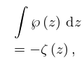
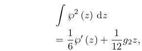
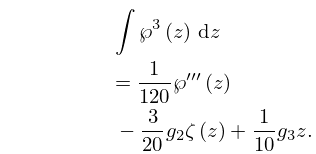
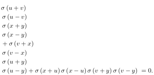
… ► … ► $\mathrm{\wp }\left(z\right)$ and $\zeta \left(z\right)$ are meromorphic functions with poles at the lattice points. $\mathrm{\wp }\left(z\right)$ is even and $\zeta \left(z\right)$ is odd. …The function $\sigma \left(z\right)$ is entire and odd, with simple zeros at the lattice points. …

7: 23.21 Physical Applications

… ►The Weierstrass function $\mathrm{\wp }$ plays a similar role for cubic potentials in canonical form $g_3+g_{2}x-4x^3$. … ►Airault et al. (1977) applies the function $\mathrm{\wp }$ to an integrable classical many-body problem, and relates the solutions to nonlinear partial differential equations. … ►where $x,y,z$ are the corresponding Cartesian coordinates and $e_1$, $e_2$, $e_3$ are constants. … ►

23.21.3 $$f(\rho )=2{\left((\rho -e_1)(\rho -e_2)(\rho -e_3)\right)}^{1/2}.$$

ⓘ

Symbols:

$e_j$: Weierstrass lattice roots, $𝕃$: lattice, $\rho$: roots and $f(\rho )$: function

Permalink:

http://dlmf.nist.gov/23.21.E3

Encodings:

pMML, png, TeX

See also:

Annotations for §23.21(iii), §23.21 and Ch.23

►Another form is obtained by identifying $e_1$, $e_2$, $e_3$ as lattice roots (§23.3(i)), and setting …

8: 23.4 Graphics

… ►

§23.4(i) Real Variables

►Line graphs of the Weierstrass functions $\mathrm{\wp }\left(x\right)$, $\zeta \left(x\right)$, and $\sigma \left(x\right)$, illustrating the lemniscatic and equianharmonic cases. … ►

►►

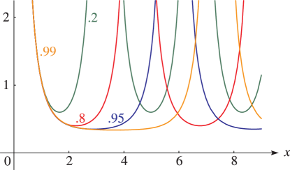
Figure 23.4.7: $\mathrm{\wp }\left(x\right)$ with ${\omega }_1=K\left(k\right)$, ${\omega }_3=\mathrm{i}{K}^{\prime }\left(k\right)$ for $0\le x\le 9$, $k^2$ = 0. … Magnify

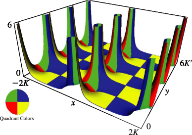
… ►Surfaces for the Weierstrass functions $\mathrm{\wp }\left(z\right)$, $\zeta \left(z\right)$, and $\sigma \left(z\right)$. … ►

►

►

Figure 23.4.8: $\mathrm{\wp }\left(x+\mathrm{i}y\right)$ with ${\omega }_1=K\left(k\right)$, ${\omega }_3=\mathrm{i}{K}^{\prime }\left(k\right)$ for $-2K\left(k\right)\le x\le 2K\left(k\right)$, $0\le y\le 6K^{\prime }\left(k\right)$, $k^2=0.9$. (The scaling makes the lattice appear to be square.) Magnify 3D Help

…

9: 23.9 Laurent and Other Power Series

… ►Let $z_0(\ne 0)$ be the nearest lattice point to the origin, and define … ►

$c_2={\displaystyle \frac{1}{20}}{g}_2,$

… ►For $j=1,2,3$, and with $e_j$ as in §23.3(i), ►

23.9.6 $$\mathrm{\wp }\left({\omega }_j+t\right)=e_j+(3{e_j}^2-5c_2)t^2+(10c_2{e}_j+21c_3)t^4+(7c_2{e_j}^2+21c_3{e}_j+5c_2^2)t^6+O\left(t^8\right),$$

ⓘ

Symbols:

$O\left(x\right)$: order not exceeding, $\mathrm{\wp }\left(z\right)$ (= $\mathrm{\wp }\left(z|𝕃\right)$ = $\mathrm{\wp }(z;g_2,g_3)$): Weierstrass $\mathrm{\wp }$-function, $e_j$: Weierstrass lattice roots, $𝕃$: lattice, ${\omega }_1$, ${\omega }_3$, ${\omega }_2=-{\omega }_1-{\omega }_3$: lattice generators, $c_n$ and $t$: variable

Referenced by:

§23.9

Permalink:

http://dlmf.nist.gov/23.9.E6

Encodings:

pMML, png, TeX

See also:

Annotations for §23.9 and Ch.23

… ►Also, Abramowitz and Stegun (1964, (18.5.25)) supplies the first 22 terms in the reverted form of (23.9.2) as $1/\mathrm{\wp }\left(z\right)\to 0$. …

10: 23.5 Special Lattices

§23.5 Special Lattices

… ►

§23.5(ii) Rectangular Lattice

… ►

§23.5(iii) Lemniscatic Lattice

… ►

§23.5(iv) Rhombic Lattice

… ►

§23.5(v) Equianharmonic Lattice

…