lattice models of critical phenomena

SearchAdvancedHelp

(0.002 seconds)

1—10 of 101 matching pages

1: 36.4 Bifurcation Sets

… ►

§36.4(i) Formulas

►

Critical Points for Cuspoids

… ►

Critical Points for Umbilics

… ►This is the codimension-one surface in $𝐱$ space where critical points coalesce, satisfying (36.4.1) and … ►This is the codimension-one surface in $𝐱$ space where critical points coalesce, satisfying (36.4.2) and …

2: 19.35 Other Applications

… ►

§19.35(ii) Physical

►Elliptic integrals appear in lattice models of critical phenomena (Guttmann and Prellberg (1993)); theories of layered materials (Parkinson (1969)); fluid dynamics (Kida (1981)); string theory (Arutyunov and Staudacher (2004)); astrophysics (Dexter and Agol (2009)). …

3: 15.18 Physical Applications

… ►The hypergeometric function has allowed the development of “solvable” models for one-dimensional quantum scattering through and over barriers (Eckart (1930), Bhattacharjie and Sudarshan (1962)), and generalized to include position-dependent effective masses (Dekar et al. (1999)). ►More varied applications include photon scattering from atoms (Gavrila (1967)), energy distributions of particles in plasmas (Mace and Hellberg (1995)), conformal field theory of critical phenomena (Burkhardt and Xue (1991)), quantum chromo-dynamics (Atkinson and Johnson (1988)), and general parametrization of the effective potentials of interaction between atoms in diatomic molecules (Herrick and O’Connor (1998)).

4: 16.24 Physical Applications

… ►

§16.24(i) Random Walks

►Generalized hypergeometric functions and Appell functions appear in the evaluation of the so-called Watson integrals which characterize the simplest possible lattice walks. They are also potentially useful for the solution of more complicated restricted lattice walk problems, and the 3D Ising model; see Barber and Ninham (1970, pp. 147–148). …

5: Sidebar 22.SB1: Decay of a Soliton in a Bose–Einstein Condensate

… ►Jacobian elliptic functions arise as solutions to certain nonlinear Schrödinger equations, which model many types of wave propagation phenomena. …This image presents the results of a computer simulation of this phenomena carried out at NIST. … ►For technical details of the physical phenomena, see B. …

6: 26.20 Physical Applications

… ►The latter reference also describes chemical applications of other combinatorial techniques. ►Applications of combinatorics, especially integer and plane partitions, to counting lattice structures and other problems of statistical mechanics, of which the Ising model is the principal example, can be found in Montroll (1964), Godsil et al. (1995), Baxter (1982), and Korepin et al. (1993). …

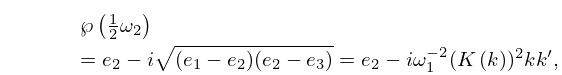
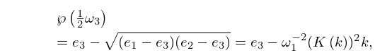
7: 23.7 Quarter Periods

… ►

23.7.1 $$\mathrm{\wp }\left(\frac{1}{2}{\omega }_1\right)=e_1+\sqrt{(e_1-e_3)(e_1-e_2)}=e_1+{\omega }_1^{-2}{(K\left(k\right))}^2{k}^{\prime },$$

ⓘ

Symbols:

$\mathrm{\wp }\left(z\right)$ (= $\mathrm{\wp }\left(z|𝕃\right)$ = $\mathrm{\wp }(z;g_2,g_3)$): Weierstrass $\mathrm{\wp }$-function, $e_j$: Weierstrass lattice roots, $K\left(k\right)$: Legendre’s complete elliptic integral of the first kind, $𝕃$: lattice, ${\omega }_1$, ${\omega }_3$, ${\omega }_2=-{\omega }_1-{\omega }_3$: lattice generators, $k$: modulus and $k^{\prime }$: complementary modulus

A&S Ref:

18.3.18

Permalink:

http://dlmf.nist.gov/23.7.E1

Encodings:

pMML, png, TeX

See also:

Annotations for §23.7 and Ch.23

►

23.7.2 $$\mathrm{\wp }\left(\frac{1}{2}{\omega }_2\right)=e_2-\mathrm{i}\sqrt{(e_1-e_2)(e_2-e_3)}=e_2-\mathrm{i}{\omega }_1^{-2}{(K\left(k\right))}^{2}k{k}^{\prime },$$

ⓘ

Symbols:

$\mathrm{\wp }\left(z\right)$ (= $\mathrm{\wp }\left(z|𝕃\right)$ = $\mathrm{\wp }(z;g_2,g_3)$): Weierstrass $\mathrm{\wp }$-function, $e_j$: Weierstrass lattice roots, $K\left(k\right)$: Legendre’s complete elliptic integral of the first kind, $\mathrm{i}$: imaginary unit, $𝕃$: lattice, ${\omega }_1$, ${\omega }_3$, ${\omega }_2=-{\omega }_1-{\omega }_3$: lattice generators, $k$: modulus and $k^{\prime }$: complementary modulus

A&S Ref:

18.3.18

Permalink:

http://dlmf.nist.gov/23.7.E2

Encodings:

pMML, png, TeX

See also:

Annotations for §23.7 and Ch.23

►

23.7.3 $$\mathrm{\wp }\left(\frac{1}{2}{\omega }_3\right)=e_3-\sqrt{(e_1-e_3)(e_2-e_3)}=e_3-{\omega }_1^{-2}{(K\left(k\right))}^{2}k,$$

ⓘ

Symbols:

$\mathrm{\wp }\left(z\right)$ (= $\mathrm{\wp }\left(z|𝕃\right)$ = $\mathrm{\wp }(z;g_2,g_3)$): Weierstrass $\mathrm{\wp }$-function, $e_j$: Weierstrass lattice roots, $K\left(k\right)$: Legendre’s complete elliptic integral of the first kind, $𝕃$: lattice, ${\omega }_1$, ${\omega }_3$, ${\omega }_2=-{\omega }_1-{\omega }_3$: lattice generators and $k$: modulus

A&S Ref:

18.3.18

Permalink:

http://dlmf.nist.gov/23.7.E3

Encodings:

pMML, png, TeX

See also:

Annotations for §23.7 and Ch.23

►where $k,k^{\prime }$ and the square roots are real and positive when the lattice is rectangular; otherwise they are determined by continuity from the rectangular case.

8: 23.3 Differential Equations

… ►The lattice invariants are defined by … ►The lattice roots satisfy the cubic equation …and are denoted by $e_1,e_2,e_3$. … ►Let $g_2^3\ne 27g_3^2$, or equivalently $\mathrm{\Delta }$ be nonzero, or $e_1,e_2,e_3$ be distinct. … ►Conversely, $g_2$, $g_3$, and the set $\{e_1,e_2,e_3\}$ are determined uniquely by the lattice $𝕃$ independently of the choice of generators. …

9: 23.14 Integrals

… ►

23.14.1 $$\int \mathrm{\wp }\left(z\right)dz=-\zeta \left(z\right),$$

ⓘ

Symbols:

$\mathrm{\wp }\left(z\right)$ (= $\mathrm{\wp }\left(z|𝕃\right)$ = $\mathrm{\wp }(z;g_2,g_3)$): Weierstrass $\mathrm{\wp }$-function, $\zeta \left(z\right)$ (= $\zeta \left(z|𝕃\right)$ = $\zeta (z;g_2,g_3)$): Weierstrass zeta function, $dx$: differential of $x$ , $\int$: integral, $𝕃$: lattice and $z$: complex

A&S Ref:

18.6.1

Permalink:

http://dlmf.nist.gov/23.14.E1

Encodings:

pMML, png, TeX

See also:

Annotations for §23.14 and Ch.23

►

23.14.2 $$\int {\mathrm{\wp }}^2\left(z\right)dz=\frac{1}{6}{\mathrm{\wp }}^{\prime }\left(z\right)+\frac{1}{12}{g}_{2}z,$$

ⓘ

Symbols:

$\mathrm{\wp }\left(z\right)$ (= $\mathrm{\wp }\left(z|𝕃\right)$ = $\mathrm{\wp }(z;g_2,g_3)$): Weierstrass $\mathrm{\wp }$-function, $g_j$: Weierstrass lattice invariants $g_2$, $g_3$ , $dx$: differential of $x$ , $\int$: integral, $𝕃$: lattice and $z$: complex

A&S Ref:

18.7.1

Permalink:

http://dlmf.nist.gov/23.14.E2

Encodings:

pMML, png, TeX

See also:

Annotations for §23.14 and Ch.23

►

23.14.3 $$\int {\mathrm{\wp }}^3\left(z\right)dz=\frac{1}{120}{\mathrm{\wp }}^{\prime \prime \prime }\left(z\right)-\frac{3}{20}{g}_2\zeta \left(z\right)+\frac{1}{10}{g}_{3}z.$$

ⓘ

Symbols:

$\mathrm{\wp }\left(z\right)$ (= $\mathrm{\wp }\left(z|𝕃\right)$ = $\mathrm{\wp }(z;g_2,g_3)$): Weierstrass $\mathrm{\wp }$-function, $g_j$: Weierstrass lattice invariants $g_2$, $g_3$ , $\zeta \left(z\right)$ (= $\zeta \left(z|𝕃\right)$ = $\zeta (z;g_2,g_3)$): Weierstrass zeta function, $dx$: differential of $x$ , $\int$: integral, $𝕃$: lattice and $z$: complex

A&S Ref:

18.7.2

Permalink:

http://dlmf.nist.gov/23.14.E3

Encodings:

pMML, png, TeX

See also:

Annotations for §23.14 and Ch.23

…

10: 23.10 Addition Theorems and Other Identities

… ►

23.10.4 $$\sigma \left(u+v\right)\sigma \left(u-v\right)\sigma \left(x+y\right)\sigma \left(x-y\right)+\sigma \left(v+x\right)\sigma \left(v-x\right)\sigma \left(u+y\right)\sigma \left(u-y\right)+\sigma \left(x+u\right)\sigma \left(x-u\right)\sigma \left(v+y\right)\sigma \left(v-y\right)=0.$$

ⓘ

Symbols:

$\sigma \left(z\right)$ (= $\sigma \left(z|𝕃\right)$ = $\sigma (z;g_2,g_3)$): Weierstrass sigma function, $𝕃$: lattice, $x$: real part of $z$ and $y$: imaginary part of $z$

Permalink:

http://dlmf.nist.gov/23.10.E4

Encodings:

pMML, png, TeX

See also:

Annotations for §23.10(i), §23.10 and Ch.23

►For further addition-type identities for the $\sigma$-function see Lawden (1989, §6.4). … ►

23.10.8 $$(\mathrm{\wp }\left(2z\right)-e_1)\mathrm{\wp }_{}^{\prime }{}_{}{}^2(z)={\left({(\mathrm{\wp }\left(z\right)-e_1)}^2-(e_1-e_2)(e_1-e_3)\right)}^2.$$

ⓘ

Symbols:

$\mathrm{\wp }\left(z\right)$ (= $\mathrm{\wp }\left(z|𝕃\right)$ = $\mathrm{\wp }(z;g_2,g_3)$): Weierstrass $\mathrm{\wp }$-function, $e_j$: Weierstrass lattice roots, $𝕃$: lattice and $z$: complex

Referenced by:

§23.10(ii), §23.10(ii)

Permalink:

http://dlmf.nist.gov/23.10.E8

Encodings:

pMML, png, TeX

See also:

Annotations for §23.10(ii), §23.10 and Ch.23

►(23.10.8) continues to hold when $e_1$, $e_2$, $e_3$ are permuted cyclically. … ►Also, when $𝕃$ is replaced by $c𝕃$ the lattice invariants $g_2$ and $g_3$ are divided by $c^4$ and $c^6$, respectively. …