Rogers–Fine identity

SearchAdvancedHelp

(0.001 seconds)

11—20 of 153 matching pages

11: 16.4 Argument Unity

… ►See Erdélyi et al. (1953a, §4.4(4)) for a non-terminating balanced identity. … ►

Rogers–Dougall Very Well-Poised Sum

… ►

§16.4(iii) Identities

… ►Methods of deriving such identities are given by Bailey (1964), Rainville (1960), Raynal (1979), and Wilson (1978). … ► …

12: 17.16 Mathematical Applications

… ►More recent applications are given in Gasper and Rahman (2004, Chapter 8) and Fine (1988, Chapters 1 and 2).

13: 17 q-Hypergeometric and Related Functions

…

14: Bibliography B

… ►

Rogers-Ramanujan identities in the hard hexagon model. J. Statist. Phys. 26 (3), pp. 427–452.

ⓘ

External Links:

ISSN 0022-4715, Document, MathReview, ZentralBlatt

Referenced by:

§17.17.

Encodings:

BibTeX

… ►

Rogers-Ramanujan Identities: A Century of Progress from Mathematics to Physics. In Proceedings of the International Congress of Mathematicians, Vol. III (Berlin, 1998), pp. 163–172.

ⓘ

External Links:

ISSN 1431-0643, FullText, MathReview (Anne Schilling), ZentralBlatt

Referenced by:

§17.17.

Encodings:

BibTeX

… ►

Phase-space projection identities for diffraction catastrophes. J. Phys. A 13 (1), pp. 149–160.

ⓘ

External Links:

ISSN 0305-4470, Document, MathReview (J. S. Joel), ZentralBlatt

Referenced by:

§36.9.

Encodings:

BibTeX

… ►

A cubic counterpart of Jacobi’s identity and the AGM. Trans. Amer. Math. Soc. 323 (2), pp. 691–701.

ⓘ

External Links:

ISSN 0002-9947, FullText, MathReview (Bruce C. Berndt), ZentralBlatt

Referenced by:

§15.8(v).

Encodings:

BibTeX

… ►

The hypergeometric identities of Cayley, Orr, and Bailey. Proc. London Math. Soc. (2) 50, pp. 56–74.

ⓘ

External Links:

Document, MathReview (N. A. Hall), ZentralBlatt

Referenced by:

§15.16.

Encodings:

BibTeX

…

15: Bibliography L

… ►

Lie algebraic approaches to classical partition identities. Adv. in Math. 29 (1), pp. 15–59.

ⓘ

External Links:

ISSN 0001-8708, Document, MathReview (S. I. Gel’fand), ZentralBlatt

Referenced by:

§17.16.

Encodings:

BibTeX

►

A Lie theoretic interpretation and proof of the Rogers-Ramanujan identities. Adv. in Math. 45 (1), pp. 21–72.

ⓘ

External Links:

ISSN 0001-8708, Document, MathReview (George E. Andrews), ZentralBlatt

Referenced by:

§17.16.

Encodings:

BibTeX

…

16: Guide to Searching the DLMF

… ►

Fine Points in Math Search

… ►

Table 3: A sample of recognized symbols

► ►►►

Symbols	Comments
…
-=	For equivalence $\equiv$
…

►

…

17: 33.22 Particle Scattering and Atomic and Molecular Spectra

… ►

§33.22(i) Schrödinger Equation

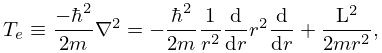
►With $\mathrm{e}$ denoting here the elementary charge, the Coulomb potential between two point particles with charges $Z_1\mathrm{e},Z_2\mathrm{e}$ and masses $m_1,m_2$ separated by a distance $s$ is $V(s)=Z_1{Z}_2{\mathrm{e}}^2/(4\pi {\epsilon }_{0}s)=Z_1{Z}_2\alpha \mathrm{\hslash }c/s$, where $Z_j$ are atomic numbers, ${\epsilon }_0$ is the electric constant, $\alpha$ is the fine structure constant, and $\mathrm{\hslash }$ is the reduced Planck’s constant. … ►

$Z=m{Z}_1{Z}_2\alpha c/\mathrm{\hslash },$

… ►For $Z_1{Z}_2=-1$ and $m=m_{\mathrm{e}}$, the electron mass, the scaling factors in (33.22.5) reduce to the Bohr radius, $a_0=\mathrm{\hslash }/(m_{\mathrm{e}}c\alpha )$, and to a multiple of the Rydberg constant, ► $R_{\mathrm{\infty }}=m_{\mathrm{e}}c{\alpha }^2/(2\mathrm{\hslash })$. …

18: 18.39 Applications in the Physical Sciences

… ►

18.39.22 $$T_e\equiv \frac{-{\mathrm{\hslash }}^2}{2m}{\nabla }^2=-\frac{{\mathrm{\hslash }}^2}{2m}\frac{1}{r^2}\frac{d}{dr}{r}^2\frac{d}{dr}+\frac{{\mathrm{L}}^2}{2m{r}^2},$$

ⓘ

Symbols:

$\frac{df}{dx}$: derivative of $f$ with respect to $x$ , $\equiv$: equals by definition and $m$: nonnegative integer

Permalink:

http://dlmf.nist.gov/18.39.E22

Encodings:

pMML, png, TeX

See also:

Annotations for §18.39(ii), §18.39 and Ch.18

… ►In what follows the radial and spherical radial eigenfunctions corresponding to (18.39.27) are found in four different notations, with identical eigenvalues, all of which appear in the current and past mathematical and theoretical physics and chemistry literatures, regarding this central problem. … ►A relativistic treatment becoming necessary as $Z$ becomes large as corrections to the non-relativistic Schrödinger picture are of approximate order ${\left(\alpha Z\right)}^2\sim {\left(Z/137\right)}^2$, $\alpha$ being the dimensionless fine structure constant $e^2/(4\pi {\epsilon }_0\mathrm{\hslash }c)$, where $c$ is the speed of light. … ►which corresponds to the exact results, in terms of Whittaker functions, of §§33.2 and 33.14, in the sense that projections onto the functions ${\varphi }_{n,l}(sr)/r$, the functions bi-orthogonal to ${\varphi }_{n,l}(sr)$, are identical. …

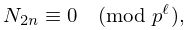
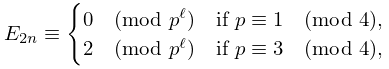
19: 24.10 Arithmetic Properties

… ►where $m\equiv n\cancel{\equiv }0(modp-1)$. …valid when $m\equiv n(mod(p-1)p^{\mathrm{\ell }})$ and $n\cancel{\equiv }0(modp-1)$, where $\mathrm{\ell }(\ge 0)$ is a fixed integer. … ►

24.10.8 $$N_{2n}\equiv 0(mod{p}^{\mathrm{\ell }}),$$

ⓘ

Symbols:

$\equiv$: modular equivalence, $\mathrm{\ell }$: integer, $n$: integer and $p$: prime

Referenced by:

§24.10(iv)

Permalink:

http://dlmf.nist.gov/24.10.E8

Encodings:

pMML, png, TeX

See also:

Annotations for §24.10(iv), §24.10 and Ch.24

►valid for fixed integers $\mathrm{\ell }(\ge 1)$, and for all $n(\ge 1)$ such that $2n\cancel{\equiv }0$ $(modp-1)$ and $p^{\mathrm{\ell }}|2n$. ►

24.10.9

ⓘ

Symbols:

$E_n$: Euler numbers, $\equiv$: modular equivalence, $\mathrm{\ell }$: integer, $n$: integer and $p$: prime

Referenced by:

§24.10(iv)

Permalink:

http://dlmf.nist.gov/24.10.E9

Encodings:

pMML, png, TeX

See also:

Annotations for §24.10(iv), §24.10 and Ch.24

…

20: 27.16 Cryptography

… ►Thus, $y\equiv x^r(modn)$ and . … ►By the Euler–Fermat theorem (27.2.8), $x^{\varphi \left(n\right)}\equiv 1(modn)$; hence $x^{t\varphi \left(n\right)}\equiv 1(modn)$. But $y^s\equiv x^{rs}\equiv x^{1+t\varphi \left(n\right)}\equiv x(modn)$, so $y^s$ is the same as $x$ modulo $n$. …