Heun functions

SearchAdvancedHelp

(0.002 seconds)

1—10 of 38 matching pages

1: 31.1 Special Notation

… ► ►►

$x$, $y$	real variables.
…

►The main functions treated in this chapter are $H\mathrm{\ell }(a,q;\alpha ,\beta ,\gamma ,\delta ;z)$, $(s_1,s_2){\mathrm{𝐻𝑓}}_m(a,q_m;\alpha ,\beta ,\gamma ,\delta ;z)$, $(s_1,s_2){\mathrm{𝐻𝑓}}_m^{\nu }(a,q_m;\alpha ,\beta ,\gamma ,\delta ;z)$, and the polynomial ${\mathrm{𝐻𝑝}}_{n,m}(a,q_{n,m};-n,\beta ,\gamma ,\delta ;z)$. …Sometimes the parameters are suppressed.

2: 31.4 Solutions Analytic at Two Singularities: Heun Functions

§31.4 Solutions Analytic at Two Singularities: Heun Functions

… ►To emphasize this property this set of functions is denoted by ►

31.4.1 $$(0,1){\mathrm{𝐻𝑓}}_m(a,q_m;\alpha ,\beta ,\gamma ,\delta ;z),$$ $m=0,1,2,\mathrm{\dots }$.

ⓘ

Symbols:

$(s_1,s_2){\mathrm{𝐻𝑓}}_m(a,q_m;\alpha ,\beta ,\gamma ,\delta ;z)$: Heun functions, $z$: complex variable, $\gamma$: real or complex parameter, $\delta$: real or complex parameter, $m$: nonnegative integer, $a$: complex parameter, $q$: real or complex parameter, $\alpha$: real or complex parameter and $\beta$: real or complex parameter

Referenced by:

§31.6

Permalink:

http://dlmf.nist.gov/31.4.E1

Encodings:

pMML, png, TeX

See also:

Annotations for §31.4 and Ch.31

… ►

31.4.3 $$(s_1,s_2){\mathrm{𝐻𝑓}}_m(a,q_m;\alpha ,\beta ,\gamma ,\delta ;z),$$ $m=0,1,2,\mathrm{\dots }$,

ⓘ

Symbols:

$(s_1,s_2){\mathrm{𝐻𝑓}}_m(a,q_m;\alpha ,\beta ,\gamma ,\delta ;z)$: Heun functions, $z$: complex variable, $\gamma$: real or complex parameter, $\delta$: real or complex parameter, $m$: nonnegative integer, $a$: complex parameter, $q$: real or complex parameter, $\alpha$: real or complex parameter and $\beta$: real or complex parameter

Referenced by:

§31.4, §31.6

Permalink:

http://dlmf.nist.gov/31.4.E3

Encodings:

pMML, png, TeX

See also:

Annotations for §31.4 and Ch.31

… ►The solutions (31.4.3) are called the Heun functions. …

3: 31.6 Path-Multiplicative Solutions

… ►A further extension of the notation (31.4.1) and (31.4.3) is given by ►

31.6.1 $$(s_1,s_2){\mathrm{𝐻𝑓}}_m^{\nu }(a,q_m;\alpha ,\beta ,\gamma ,\delta ;z),$$ $m=0,1,2,\mathrm{\dots }$,

ⓘ

Symbols:

$(s_1,s_2){\mathrm{𝐻𝑓}}_m(a,q_m;\alpha ,\beta ,\gamma ,\delta ;z)$: Heun functions, $z$: complex variable, $\gamma$: real or complex parameter, $\delta$: real or complex parameter, $\nu$: real or complex parameter, $m$: nonnegative integer, $a$: complex parameter, $q$: real or complex parameter, $\alpha$: real or complex parameter, $\beta$: real or complex parameter and $s_j$: parameters

Permalink:

http://dlmf.nist.gov/31.6.E1

Encodings:

pMML, png, TeX

See also:

Annotations for §31.6 and Ch.31

…

4: 31 Heun Functions

Chapter 31 Heun Functions

…

5: 31.9 Orthogonality

… ►

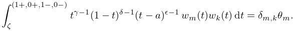
§31.9(i) Single Orthogonality

… ►

31.9.1 $$w_m(z)=(0,1){\mathrm{𝐻𝑓}}_m(a,q_m;\alpha ,\beta ,\gamma ,\delta ;z),$$

ⓘ

Symbols:

$(s_1,s_2){\mathrm{𝐻𝑓}}_m(a,q_m;\alpha ,\beta ,\gamma ,\delta ;z)$: Heun functions, $z$: complex variable, $\gamma$: real or complex parameter, $\delta$: real or complex parameter, $m$: nonnegative integer, $a$: complex parameter, $q$: real or complex parameter, $\alpha$: real or complex parameter and $\beta$: real or complex parameter

Permalink:

http://dlmf.nist.gov/31.9.E1

Encodings:

pMML, png, TeX

See also:

Annotations for §31.9(i), §31.9 and Ch.31

… ►

31.9.2 $${\int }_{\zeta }^{(1+,0+,1-,0-)}{t}^{\gamma -1}{(1-t)}^{\delta -1}{(t-a)}^{ϵ-1}{w}_m(t)w_k(t)dt={\delta }_{m,k}{\theta }_m.$$

ⓘ

Symbols:

${\delta }_{j,k}$: Kronecker delta, $dx$: differential of $x$ , $\int$: integral, $\gamma$: real or complex parameter, $\delta$: real or complex parameter, $ϵ$: real or complex parameter, $m$: nonnegative integer, $a$: complex parameter, $\zeta$: point and ${\theta }_m$: normalization constant

Permalink:

http://dlmf.nist.gov/31.9.E2

Encodings:

pMML, png, TeX

See also:

Annotations for §31.9(i), §31.9 and Ch.31

… ►For corresponding orthogonality relations for Heun functions (§31.4) and Heun polynomials (§31.5), see Lambe and Ward (1934), Erdélyi (1944), Sleeman (1966a), and Ronveaux (1995, Part A, pp. 59–64). ►

§31.9(ii) Double Orthogonality

…

6: 31.18 Methods of Computation

§31.18 Methods of Computation

… ►The computation of the accessory parameter for the Heun functions is carried out via the continued-fraction equations (31.4.2) and (31.11.13) in the same way as for the Mathieu, Lamé, and spheroidal wave functions in Chapters 28–30.

7: 31.17 Physical Applications

§31.17 Physical Applications

… ►

§31.17(ii) Other Applications

►Heun functions appear in the theory of black holes (Kerr (1963), Teukolsky (1972), Chandrasekhar (1984), Suzuki et al. (1998), Kalnins et al. (2000)), lattice systems in statistical mechanics (Joyce (1973, 1994)), dislocation theory (Lay and Slavyanov (1999)), and solution of the Schrödinger equation of quantum mechanics (Bay et al. (1997), Tolstikhin and Matsuzawa (2001), and Hall et al. (2010)). … ►More applications—including those of generalized spheroidal wave functions and confluent Heun functions in mathematical physics, astrophysics, and the two-center problem in molecular quantum mechanics—can be found in Leaver (1986) and Slavyanov and Lay (2000, Chapter 4). …

8: 31.10 Integral Equations and Representations

… ►

Kernel Functions

… ►Then the integral equation (31.10.1) is satisfied by $w(z)=w_m(z)$ and $W(z)={\kappa }_m{w}_m(z)$, where $w_m(z)=(0,1){\mathrm{𝐻𝑓}}_m(a,q_m;\alpha ,\beta ,\gamma ,\delta ;z)$ and ${\kappa }_m$ is the corresponding eigenvalue. … ►Fuchs–Frobenius solutions $W_m(z)={\tilde{\kappa }}_m{z}^{-\alpha }H\mathrm{\ell }(1/a,q_m;\alpha ,\alpha -\gamma +1,\alpha -\beta +1,\delta ;1/z)$ are represented in terms of Heun functions $w_m(z)=(0,1){\mathrm{𝐻𝑓}}_m(a,q_m;\alpha ,\beta ,\gamma ,\delta ;z)$ by (31.10.1) with $W(z)=W_m(z)$, $w(z)=w_m(z)$, and with kernel chosen from … ►

Kernel Functions

… ►For integral equations for special confluent Heun functions (§31.12) see Kazakov and Slavyanov (1996). …

9: 31.13 Asymptotic Approximations

§31.13 Asymptotic Approximations

…

10: 31.7 Relations to Other Functions

… ►

§31.7(i) Reductions to the Gauss Hypergeometric Function

… ►

31.7.2 $$H\mathrm{\ell }(2,\alpha \beta ;\alpha ,\beta ,\gamma ,\alpha +\beta -2\gamma +1;z)={}_2{}^{}F_1^{}(\frac{1}{2}\alpha ,\frac{1}{2}\beta ;\gamma ;1-{(1-z)}^2),$$

ⓘ

Symbols:

${}_2{}^{}F_1^{}(a,b;c;z)$: $=F(a,b;c;z)$ notation for Gauss’ hypergeometric function, $H\mathrm{\ell }(a,q;\alpha ,\beta ,\gamma ,\delta ;z)$: Heun functions, $z$: complex variable, $\gamma$: real or complex parameter, $\alpha$: real or complex parameter and $\beta$: real or complex parameter

Permalink:

http://dlmf.nist.gov/31.7.E2

Encodings:

pMML, png, TeX

See also:

Annotations for §31.7(i), §31.7 and Ch.31

►

31.7.3 $$H\mathrm{\ell }(4,\alpha \beta ;\alpha ,\beta ,\frac{1}{2},\frac{2}{3}(\alpha +\beta );z)={}_2{}^{}F_1^{}(\frac{1}{3}\alpha ,\frac{1}{3}\beta ;\frac{1}{2};1-{(1-z)}^2(1-\frac{1}{4}z)),$$

ⓘ

Symbols:

${}_2{}^{}F_1^{}(a,b;c;z)$: $=F(a,b;c;z)$ notation for Gauss’ hypergeometric function, $H\mathrm{\ell }(a,q;\alpha ,\beta ,\gamma ,\delta ;z)$: Heun functions, $z$: complex variable, $\alpha$: real or complex parameter and $\beta$: real or complex parameter

Permalink:

http://dlmf.nist.gov/31.7.E3

Encodings:

pMML, png, TeX

See also:

Annotations for §31.7(i), §31.7 and Ch.31

►

31.7.4 $$H\mathrm{\ell }(\frac{1}{2}+\mathrm{i}\frac{\sqrt{3}}{2},\alpha \beta (\frac{1}{2}+\mathrm{i}\frac{\sqrt{3}}{6});\alpha ,\beta ,\frac{1}{3}(\alpha +\beta +1),\frac{1}{3}(\alpha +\beta +1);z)={}_2{}^{}F_1^{}(\frac{1}{3}\alpha ,\frac{1}{3}\beta ;\frac{1}{3}(\alpha +\beta +1);1-{\left(1-\left(\frac{3}{2}-\mathrm{i}\frac{\sqrt{3}}{2}\right)z\right)}^3).$$

ⓘ

Symbols:

${}_2{}^{}F_1^{}(a,b;c;z)$: $=F(a,b;c;z)$ notation for Gauss’ hypergeometric function, $H\mathrm{\ell }(a,q;\alpha ,\beta ,\gamma ,\delta ;z)$: Heun functions, $\mathrm{i}$: imaginary unit, $z$: complex variable, $\alpha$: real or complex parameter and $\beta$: real or complex parameter

Permalink:

http://dlmf.nist.gov/31.7.E4

Encodings:

pMML, png, TeX

See also:

Annotations for §31.7(i), §31.7 and Ch.31

… ►

§31.7(ii) Relations to Lamé Functions

…