.巴西对塞尔维亚世界杯_『wn4.com_』世界杯ipad用啥看_w6n2c9o_2022年11月30日1时9分10秒_n1z1jllvb_gov_hk

(0.006 seconds)

11—20 of 804 matching pages

11: 24.20 Tables

… ►Abramowitz and Stegun (1964, Chapter 23) includes exact values of

\sum_{k=1}^{m}k^{n}

m=1(1)100

n=1(1)10

;

\sum_{k=1}^{\infty}k^{-n}

\sum_{k=1}^{\infty}(-1)^{k-1}k^{-n}

\sum_{k=0}^{\infty}(2k+1)^{-n}

n=1,2,\dotsc

, 20D;

\sum_{k=0}^{\infty}(-1)^{k}(2k+1)^{-n}

n=1,2,\dotsc

, 18D. ►Wagstaff (1978) gives complete prime factorizations of

N_{n}

and

E_{n}

for

n=20(2)60

and

n=8(2)42

, respectively. … ►For information on tables published before 1961 see Fletcher et al. (1962, v. 1, §4) and Lebedev and Fedorova (1960, Chapters 11 and 14).

12: 26.4 Lattice Paths: Multinomial Coefficients and Set Partitions

… ►

\genfrac{(}{)}{0.0pt}{}{n}{n_{1},n_{2},\ldots,n_{k}}

is the number of ways of placing

n=n_{1}+n_{2}+\cdots+n_{k}

distinct objects into

k

labeled boxes so that there are

n_{j}

objects in the

j

th box. … ►These are given by the following equations in which

a_{1},a_{2},\ldots,a_{n}

are nonnegative integers such that …

M_{1}

is the multinominal coefficient (26.4.2): …For each

n

all possible values of

a_{1},a_{2},\ldots,a_{n}

are covered. … ►where the summation is over all nonnegative integers

n_{1},n_{2},\ldots,n_{k}

such that

n_{1}+n_{2}+\cdots+n_{k}=n

. …

13: 26.16 Multiset Permutations

… ►Let

S=\{1^{a_{1}},2^{a_{2}},\ldots,n^{a_{n}}\}

be the multiset that has

a_{j}

copies of

j

1\leq j\leq n

\mathfrak{S}_{S}

denotes the set of permutations of

S

for all distinct orderings of the

a_{1}+a_{2}+\cdots+a_{n}

integers. The number of elements in

\mathfrak{S}_{S}

is the multinomial coefficient (§26.4)

\genfrac{(}{)}{0.0pt}{}{a_{1}+a_{2}+\cdots+a_{n}}{a_{1},a_{2},\ldots,a_{n}}

. … ►The $q$ -multinomial coefficient is defined in terms of Gaussian polynomials (§26.9(ii)) by …and again with

S=\{1^{a_{1}},2^{a_{2}},\ldots,n^{a_{n}}\}

we have …

Miller (1946) tabulates $\operatorname{Ai}\left(x\right)$ , $\operatorname{Ai}'\left(x\right)$ for $x=-20(.01)2;$ $\operatorname{log}_{10}\operatorname{Ai}\left(x\right)$ , $\operatorname{Ai}'\left(x\right)/\operatorname{Ai}\left(x\right)$ for $x=0(.1)25(1)75$ ; $\operatorname{Bi}\left(x\right)$ , $\operatorname{Bi}'\left(x\right)$ for $x=-10(.1)2.5$ ; $\operatorname{log}_{10}\operatorname{Bi}\left(x\right)$ , $\operatorname{Bi}'\left(x\right)/\operatorname{Bi}\left(x\right)$ for $x=0(.1)10$ ; $M\left(x\right)$ , $N\left(x\right)$ , $\theta\left(x\right)$ , $\phi\left(x\right)$ (respectively $F(x)$ , $G(x)$ , $\chi(x)$ , $\psi(x)$ ) for $x=-80(1)-30(.1)0$ . Precision is generally 8D; slightly less for some of the auxiliary functions. Extracts from these tables are included in Abramowitz and Stegun (1964, Chapter 10), together with some auxiliary functions for large arguments.

… ►

•

Miller (1946) tabulates $a_{k}$ , $\operatorname{Ai}'\left(a_{k}\right)$ , $a^{\prime}_{k}$ , $\operatorname{Ai}\left(a^{\prime}_{k}\right)$ , $k=1(1)50$ ; $b_{k}$ , $\operatorname{Bi}'\left(b_{k}\right)$ , $b^{\prime}_{k}$ , $\operatorname{Bi}\left(b^{\prime}_{k}\right)$ , $k=1(1)20$ . Precision is 8D. Entries for $k=1(1)20$ are reproduced in Abramowitz and Stegun (1964, Chapter 10).

… ►

•

Rothman (1954b) tabulates $\int_{0}^{x}\operatorname{Ai}\left(t\right)\,\mathrm{d}t$ and $\int_{0}^{x}\operatorname{Bi}\left(t\right)\,\mathrm{d}t$ for $x=-10(.1)\infty$ and $-10(.1)2$ , respectively; 7D. The entries in the columns headed $\int_{0}^{x}\operatorname{Ai}\left(-x\right)\,\mathrm{d}x$ and $\int_{0}^{x}\operatorname{Bi}\left(-x\right)\,\mathrm{d}x$ all have the wrong sign. The tables are reproduced in Abramowitz and Stegun (1964, Chapter 10), and the sign errors are corrected in later reprintings.

… ►

•

Zhang and Jin (1996, p. 338) tabulates $\int_{0}^{x}\operatorname{Ai}\left(t\right)\,\mathrm{d}t$ and $\int_{0}^{x}\operatorname{Bi}\left(t\right)\,\mathrm{d}t$ for $x=-10(.2)10$ to 8D or 8S.

… ►

•

National Bureau of Standards (1958) tabulates $A_{0}(x)\equiv\pi\operatorname{Hi}\left(-x\right)$ and $-A_{0}^{\prime}(x)\equiv\pi\operatorname{Hi}'\left(-x\right)$ for $x=0(.01)1(.02)5(.05)11$ and $1/x=0.01(.01)0.1$ ; $\int_{0}^{x}A_{0}(t)\,\mathrm{d}t$ for $x=0.5,1(1)11$ . Precision is 8D.

…

16: 34.1 Special Notation

… ►

\begin{pmatrix}j_{1}&j_{2}&j_{3}\\ m_{1}&m_{2}&m_{3}\end{pmatrix},

►

\begin{Bmatrix}j_{1}&j_{2}&j_{3}\\ l_{1}&l_{2}&l_{3}\end{Bmatrix},

►

\begin{Bmatrix}j_{11}&j_{12}&j_{13}\\ j_{21}&j_{22}&j_{23}\\ j_{31}&j_{32}&j_{33}\end{Bmatrix}.

►An often used alternative to the

\mathit{3j}

symbol is the Clebsch–Gordan coefficient ►

34.1.1

\left(j_{1}\;m_{1}\;j_{2}\;m_{2}|j_{1}\;j_{2}\;j_{3}\,\,m_{3}\right)=(-1)^{j_{% 1}-j_{2}+m_{3}}(2j_{3}+1)^{\frac{1}{2}}\begin{pmatrix}j_{1}&j_{2}&j_{3}\\ m_{1}&m_{2}&-m_{3}\end{pmatrix};

ⓘ

Symbols:: $\begin{pmatrix}\NVar{j_{1}}&\NVar{j_{2}}&\NVar{j_{3}}\\ \NVar{m_{1}}&\NVar{m_{2}}&\NVar{m_{3}}\end{pmatrix}$ : $\mathit{3j}$ symbol and $j,j_{r}$ : non-negative integers or non-negative integers plus one half.
Sources:: Edmonds (1974, p. 46, Eq. (3.7.3)); Rotenberg et al. (1959, p. 1, Eq. (1.1a))
Permalink:: http://dlmf.nist.gov/34.1.E1
Encodings:: pMML, png, TeX
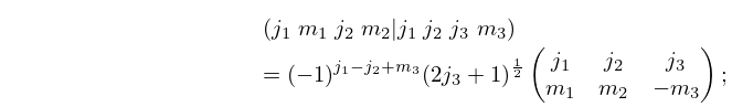
Clarification (effective with 1.0.15):: A wording change reflects that the Clebsch–Gordan coefficients are an alternative formulation of angular momentum problems, rather than alternative notation for the $\mathit{3j}$ . The sign of $m_{3}$ was changed for clarity.
See also:: Annotations for §34.1 and Ch.34

…

17: 34.3 Basic Properties: $\mathit{3j}$ Symbol

… ►When any one of

j_{1},j_{2},j_{3}

is equal to

0,\tfrac{1}{2}

, or

1

, the

\mathit{3j}

symbol has a simple algebraic form. …For these and other results, and also cases in which any one of

j_{1},j_{2},j_{3}

\frac{3}{2}

2

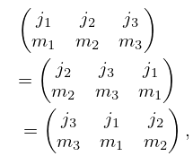
, see Edmonds (1974, pp. 125–127). … ►Even permutations of columns of a

\mathit{3j}

symbol leave it unchanged; odd permutations of columns produce a phase factor

(-1)^{j_{1}+j_{2}+j_{3}}

, for example, ►

34.3.8

\begin{pmatrix}j_{1}&j_{2}&j_{3}\\ m_{1}&m_{2}&m_{3}\end{pmatrix}=\begin{pmatrix}j_{2}&j_{3}&j_{1}\\ m_{2}&m_{3}&m_{1}\end{pmatrix}=\begin{pmatrix}j_{3}&j_{1}&j_{2}\\ m_{3}&m_{1}&m_{2}\end{pmatrix},

ⓘ

Symbols:: $\begin{pmatrix}\NVar{j_{1}}&\NVar{j_{2}}&\NVar{j_{3}}\\ \NVar{m_{1}}&\NVar{m_{2}}&\NVar{m_{3}}\end{pmatrix}$ : $\mathit{3j}$ symbol and $j,j_{r}$ : non-negative integers or non-negative integers plus one half.
Referenced by:: §34.3(ii)
Permalink:: http://dlmf.nist.gov/34.3.E8
Encodings:: pMML, png, TeX
See also:: Annotations for §34.3(ii), §34.3 and Ch.34

… ►For the polynomials

P_{l}

see §18.3, and for the function

Y_{{l},{m}}

see §14.30. …

18: 18.8 Differential Equations

… ►

Table 18.8.1: Classical OP’s: differential equations

A(x)f^{\prime\prime}(x)+B(x)f^{\prime}(x)+C(x)f(x)+\lambda_{n}f(x)=0

► ►►►►►

#	$f(x)$	$A(x)$	$B(x)$	$C(x)$	$\lambda_{n}$
…
11	${\mathrm{e}}^{-n^{-1}x}x^{\ell+1}L^{(2\ell+1)}_{n-\ell-1}\left(2n^{-1}x\right)$	$1$	$0$	$\frac{2}{x}-\frac{\ell(\ell+1)}{x^{2}}$	$-\frac{1}{n^{2}}$
12	$H_{n}\left(x\right)$	$1$	$-2x$	$0$	$2n$
…
14	$\mathit{He}_{n}\left(x\right)$	$1$	$-x$	$0$	$n$

► ►Item 11 of Table 18.8.1 yields (18.39.36) for

Z=1

19: 1.12 Continued Fractions

… ►

A_{n}

and

B_{n}

are called the

n

th (canonical) numerator and denominator respectively. … ►

b_{0}+\displaystyle{\cfrac{a_{1}}{b_{1}+\cfrac{a_{2}}{b_{2}+\cdots}}}

is equivalent to

b^{\prime}_{0}+\displaystyle{\cfrac{a^{\prime}_{1}}{b^{\prime}_{1}+\cfrac{a^{% \prime}_{2}}{b^{\prime}_{2}+\cdots}}}

if there is a sequence

\{d_{n}\}^{\infty}_{n=0}

d_{0}=1

d_{n}\neq 0

, such that … ►Define … ►The continued fraction

\displaystyle{\cfrac{a_{1}}{b_{1}+\cfrac{a_{2}}{b_{2}+\cdots}}}

converges when … ►Then the convergents

C_{n}

satisfy …

20: 3.6 Linear Difference Equations

… ►Given numerical values of

w_{0}

and

w_{1}

, the solution

w_{n}

of the equation … ►beginning with

e_{0}=w_{0}

. … ►We apply the algorithm to compute

\mathbf{E}_{n}\left(1\right)

to 8S for the range

n=1,2,\dots,10

, beginning with the value

\mathbf{E}_{0}\left(1\right)=-0.56865\;\,663

obtained from the Maclaurin series expansion (§11.10(iii)). … ►The values of

w_{n}

for

n=1,2,\dots,10

are the wanted values of

\mathbf{E}_{n}\left(1\right)

. (It should be observed that for

n>10

, however, the

w_{n}

are progressively poorer approximations to

\mathbf{E}_{n}\left(1\right)

: the underlined digits are in error.) …

.巴西对塞尔维亚世界杯_『wn4.com_』世界杯ipad用啥看_w6n2c9o_2022年11月30日1时9分10秒_n1z1jllvb_gov_hk

11—20 of 804 matching pages

11: 24.20 Tables

12: 26.4 Lattice Paths: Multinomial Coefficients and Set Partitions

13: 26.16 Multiset Permutations

14: 30.7 Graphics

15: 9.18 Tables

16: 34.1 Special Notation

17: 34.3 Basic Properties: $\mathit{3j}$ Symbol

18: 18.8 Differential Equations

19: 1.12 Continued Fractions

20: 3.6 Linear Difference Equations

.巴西对塞尔维亚世界杯_『wn4.com_』世界杯ipad用啥看_w6n2c9o_2022年11月30日1时9分10秒_n1z1jllvb_gov_hk

11—20 of 804 matching pages

11: 24.20 Tables

12: 26.4 Lattice Paths: Multinomial Coefficients and Set Partitions

13: 26.16 Multiset Permutations

14: 30.7 Graphics

15: 9.18 Tables

16: 34.1 Special Notation

17: 34.3 Basic Properties: 3 ⁢ j Symbol

18: 18.8 Differential Equations

19: 1.12 Continued Fractions

20: 3.6 Linear Difference Equations

17: 34.3 Basic Properties: $\mathit{3j}$ Symbol