tempered%20distributions

SearchAdvancedHelp

(0.002 seconds)

11—20 of 152 matching pages

11: Errata

… ►The spectral theory of these operators, based on Sturm-Liouville and Liouville normal forms, distribution theory, is now discussed more completely, including linear algebra, matrices, matrices as linear operators, orthonormal expansions, Stieltjes integrals/measures, generating functions. … ►

Several changes have been made to

1. make consistent use of the Fourier transform notations $ℱ\left(f\right)$, $ℱ\left(\varphi \right)$ and $ℱ\left(u\right)$ where $f$ is a function of one real variable, $\varphi$ is a test function of $n$ variables associated with tempered distributions, and $u$ is a tempered distribution (see (1.14.1), (1.16.29) and (1.16.35));

2. introduce the partial differential operator $𝐃$ in (1.16.30);

3. clarify the definition (1.16.32) of the partial differential operator $P(𝐃)$; and

4. clarify the use of $P(𝐃)$ and $P(𝐱)$ in (1.16.33), (1.16.34), (1.16.36) and (1.16.37).

►

An entire new Subsection 1.16(viii) Fourier Transforms of Special Distributions, was contributed by Roderick Wong.

… ►

Several new equations have been added. See (8.17.24), (20.7.34), §20.11(v), (26.12.27), (36.2.28), and (36.2.29).

… ►

Bibliographic citations were added in §§1.13(v), 10.14, 10.21(ii), 18.15(v), 18.32, 30.16(iii), 32.13(ii), and as general references in Chapters 19, 20, 22, and 23.

…

12: 3.8 Nonlinear Equations

… ►For describing the distribution of complex zeros of solutions of linear homogeneous second-order differential equations by methods based on the Liouville–Green (WKB) approximation, see Segura (2013). … ►

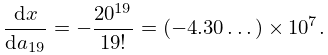
3.8.15 $$p(x)=(x-1)(x-2)\mathrm{\cdots }(x-20)$$

ⓘ

Permalink:

http://dlmf.nist.gov/3.8.E15

Encodings:

pMML, png, TeX

See also:

Annotations for §3.8(vi), §3.8(vi), §3.8 and Ch.3

… ►Consider $x=20$ and $j=19$. We have $p^{\prime }(20)=19!$ and $a_{19}=1+2+\mathrm{\cdots }+20=210$. … ►

3.8.16 $$\frac{dx}{d{a}_{19}}=-\frac{{20}^{19}}{19!}=(-4.30\mathrm{\dots })\times {10}^7.$$

ⓘ

Symbols:

$\frac{df}{dx}$: derivative of $f$ with respect to $x$ and $!$: factorial (as in $n!$)

Permalink:

http://dlmf.nist.gov/3.8.E16

Encodings:

pMML, png, TeX

See also:

Annotations for §3.8(vi), §3.8(vi), §3.8 and Ch.3

…

13: Sidebar 7.SB1: Diffraction from a Straightedge

… ►The intensity distribution follows ${|ℱ\left(x\right)|}^2$, where $ℱ$ is the Fresnel integral (See 7.3.4). …

14: Funding

… ►The NIST DLMF project has been funded, in part, by the Knowledge & Distributed Intelligence Program of the National Science Foundation. …

15: Bibliography O

… ►

Tables of Fourier Transforms and Fourier Transforms of Distributions. Springer-Verlag, Berlin.

ⓘ

External Links:

ISBN 3-540-50630-6; 0-387-50630-6, MathReview, ZentralBlatt

Referenced by:

§1.14(viii), §10.22(vi), §10.43(vi), §11.10(x), §11.7(v), §11.9(iv), §12.12, §13.10(iv), §13.23(ii), §18.17(ix), §6.14(iii), §7.14(iii).

Encodings:

BibTeX

… ►

On the distribution of spacings between zeros of the zeta function. Math. Comp. 48 (177), pp. 273–308.

ⓘ

External Links:

ISSN 0025-5718, FullText, Author’s Website, MathReview (S. L. Segal), ZentralBlatt

Referenced by:

§25.18(ii).

Encodings:

BibTeX

… ►

An error analysis of the modified Clenshaw method for evaluating Chebyshev and Fourier series. J. Inst. Math. Appl. 20 (3), pp. 379–391.

ⓘ

External Links:

Document, MathReview (David L. Elliott), ZentralBlatt

Referenced by:

§3.11(ii).

Encodings:

BibTeX

… ►

Distribution of the partition function modulo $m$ . Ann. of Math. (2) 151 (1), pp. 293–307.

ⓘ

External Links:

ISSN 0003-486X, FullText, MathReview (Bruce C. Berndt), ZentralBlatt

Referenced by:

§27.14(v).

Encodings:

BibTeX

…

16: 10.73 Physical Applications

… ►Laplace’s equation governs problems in heat conduction, in the distribution of potential in an electrostatic field, and in hydrodynamics in the irrotational motion of an incompressible fluid. … ►See Krivoshlykov (1994, Chapter 2, §2.2.10; Chapter 5, §5.2.2), Kapany and Burke (1972, Chapters 4–6; Chapter 7, §A.1), and Slater (1942, Chapter 4, §§20, 25). … ►The analysis of the current distribution in circular conductors leads to the Kelvin functions $\mathrm{ber}x$, $\mathrm{bei}x$, $\ker x$, and $\mathrm{kei}x$. …

17: 36.5 Stokes Sets

… ►

36.5.4 $$80x^5-40x^4-55x^3+5x^2+20x-1=0,$$

ⓘ

Symbols:

$x$: real parameter

Permalink:

http://dlmf.nist.gov/36.5.E4

Encodings:

pMML, png, TeX

See also:

Annotations for §36.5(ii), §36.5(ii), §36.5 and Ch.36

… ►

36.5.7 $$X=\frac{9}{20}+20u^4-\frac{Y^2}{20u^2}+6u^2\mathrm{sign}\left(z\right),$$

ⓘ

Symbols:

$\mathrm{sign}x$: sign of, $z$: real parameter, $X$: scaled coordinate and $Y$: scaled coordinate

Permalink:

http://dlmf.nist.gov/36.5.E7

Encodings:

pMML, png, TeX

See also:

Annotations for §36.5(ii), §36.5(ii), §36.5 and Ch.36

… ►The distribution of real and complex critical points in Figures 36.5.5 and 36.5.6 follows from consistency with Figure 36.5.1 and the fact that there are four real saddles in the inner regions. …

18: 8 Incomplete Gamma and Related
Functions

…

19: 28 Mathieu Functions and Hill’s Equation

…

20: 9.9 Zeros

… ►

§9.9(i) Distribution and Notation

… ►For the distribution in $ℂ$ of the zeros of ${\mathrm{Ai}}^{\prime }\left(z\right)-\sigma \mathrm{Ai}\left(z\right)$, where $\sigma$ is an arbitrary complex constant, see Muraveĭ (1976) and Gil and Segura (2014). … ►

9.9.6 $$a_k=-T\left(\frac{3}{8}\pi (4k-1)\right),$$

ⓘ

Symbols:

$\pi$: the ratio of the circumference of a circle to its diameter, $a_k$: $k$th zero of Airy $\mathrm{Ai}$ , $k$: nonnegative integer and $T$: expansion

Source:

Olver (1954, (A 20))

Permalink:

http://dlmf.nist.gov/9.9.E6

Encodings:

pMML, png, TeX

See also:

Annotations for §9.9(iv), §9.9 and Ch.9

►

9.9.7 $${\mathrm{Ai}}^{\prime }\left(a_k\right)={(-1)}^{k-1}V\left(\frac{3}{8}\pi (4k-1)\right),$$

ⓘ

Symbols:

$\mathrm{Ai}\left(z\right)$: Airy function, $\pi$: the ratio of the circumference of a circle to its diameter, $a_k$: $k$th zero of Airy $\mathrm{Ai}$ , $k$: nonnegative integer and $V$: expansion

Source:

Olver (1954, (A 20))

Permalink:

http://dlmf.nist.gov/9.9.E7

Encodings:

pMML, png, TeX

See also:

Annotations for §9.9(iv), §9.9 and Ch.9

►

9.9.8 $$a_k^{\prime }=-U\left(\frac{3}{8}\pi (4k-3)\right),$$

ⓘ

Symbols:

$\pi$: the ratio of the circumference of a circle to its diameter, $a_k^{\prime }$: $k$th zero of Airy ${\mathrm{Ai}}^{\prime }$ , $k$: nonnegative integer and $U$: expansion

Source:

Olver (1954, (A 20))

Permalink:

http://dlmf.nist.gov/9.9.E8

Encodings:

pMML, png, TeX

See also:

Annotations for §9.9(iv), §9.9 and Ch.9

…