singularity parameter

SearchAdvancedHelp

(0.002 seconds)

21—30 of 61 matching pages

21: 31.18 Methods of Computation

… ►Independent solutions of (31.2.1) can be computed in the neighborhoods of singularities from their Fuchs–Frobenius expansions (§31.3), and elsewhere by numerical integration of (31.2.1). …The computation of the accessory parameter for the Heun functions is carried out via the continued-fraction equations (31.4.2) and (31.11.13) in the same way as for the Mathieu, Lamé, and spheroidal wave functions in Chapters 28–30.

22: 12.16 Mathematical Applications

… ►PCFs are used as basic approximating functions in the theory of contour integrals with a coalescing saddle point and an algebraic singularity, and in the theory of differential equations with two coalescing turning points; see §§2.4(vi) and 2.8(vi). … ►PCFs are also used in integral transforms with respect to the parameter, and inversion formulas exist for kernels containing PCFs. …

23: 10.2 Definitions

… ►

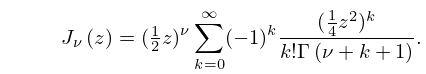
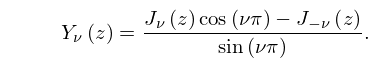
§10.2(i) Bessel’s Equation

►

10.2.1 $$z^2\frac{d^{2}w}{{dz}^2}+z\frac{dw}{dz}+(z^2-{\nu }^2)w=0.$$

ⓘ

Symbols:

$\frac{df}{dx}$: derivative of $f$ with respect to $x$ , $z$: complex variable and $\nu$: complex parameter

A&S Ref:

9.1.1

Referenced by:

§10.13, §10.15, §10.2(ii), §10.2(ii), §10.2(iii), §10.24, §10.25(i), §10.27, §10.4, §10.61(ii), §10.74(ii)

Permalink:

http://dlmf.nist.gov/10.2.E1

Encodings:

pMML, png, TeX

See also:

Annotations for §10.2(i), §10.2 and Ch.10

►This differential equation has a regular singularity at $z=0$ with indices $\pm \nu$, and an irregular singularity at $z=\mathrm{\infty }$ of rank $1$; compare §§2.7(i) and 2.7(ii). … ►

10.2.2 $$J_{\nu }\left(z\right)={(\frac{1}{2}z)}^{\nu }\sum _{k=0}^{\mathrm{\infty }}{(-1)}^k\frac{{(\frac{1}{4}{z}^2)}^k}{k!\mathrm{\Gamma }\left(\nu +k+1\right)}.$$

ⓘ

Defines:

$J_{\nu }\left(z\right)$: Bessel function of the first kind

Symbols:

$\mathrm{\Gamma }\left(z\right)$: gamma function, $!$: factorial (as in $n!$), $k$: nonnegative integer, $z$: complex variable and $\nu$: complex parameter

A&S Ref:

9.1.10

Referenced by:

§10.11, §10.16, §10.19(i), §10.22(ii), §10.22(iii), §10.24, §10.53, §10.65(i), §10.7(i), §10.74(ii), §10.8, §18.38(iii), §8.6(i)

Permalink:

http://dlmf.nist.gov/10.2.E2

Encodings:

pMML, png, TeX

See also:

Annotations for §10.2(ii), §10.2(ii), §10.2 and Ch.10

… ►

10.2.3 $$Y_{\nu }\left(z\right)=\frac{J_{\nu }\left(z\right)\cos \left(\nu \pi \right)-J_{-\nu }\left(z\right)}{\sin \left(\nu \pi \right)}.$$

ⓘ

Defines:

$Y_{\nu }\left(z\right)$: Bessel function of the second kind

Symbols:

$J_{\nu }\left(z\right)$: Bessel function of the first kind, $\pi$: the ratio of the circumference of a circle to its diameter, $\cos z$: cosine function, $\sin z$: sine function, $z$: complex variable and $\nu$: complex parameter

A&S Ref:

9.1.2

Referenced by:

§10.11, §10.15, §10.19(i), §10.2(ii), §10.22(ii), §10.24, §10.4, §10.47(ii), §10.7(i), §10.8, §11.10(v), §11.4(i)

Permalink:

http://dlmf.nist.gov/10.2.E3

Encodings:

pMML, png, TeX

See also:

Annotations for §10.2(ii), §10.2(ii), §10.2 and Ch.10

…

24: 15.10 Hypergeometric Differential Equation

… ►It has regular singularities at $z=0,1,\mathrm{\infty }$, with corresponding exponent pairs $\{0,1-c\}$, $\{0,c-a-b\}$, $\{a,b\}$, respectively. …They are also numerically satisfactory (§2.7(iv)) in the neighborhood of the corresponding singularity. ►

Singularity $z=0$

… ►

Singularity $z=1$

… ►

Singularity $z=\mathrm{\infty }$

…

25: 36.6 Scaling Relations

… ►

Indices for $k$-Scaling of Magnitude of ${\mathrm{\Psi }}_K$ or ${\mathrm{\Psi }}^{(\mathrm{U})}$ (Singularity Index)

… ►

Table 36.6.1: Special cases of scaling exponents for cuspoids.

► ►►

singularity	$K$	${\beta }_K$	${\gamma }_{1K}$	${\gamma }_{2K}$	${\gamma }_{3K}$	${\gamma }_K$
…

►

…

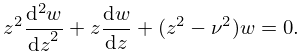
26: 31.3 Basic Solutions

… ►

31.3.2 $$a\gamma c_1-q{c}_0=0,$$

ⓘ

Symbols:

$\gamma$: real or complex parameter, $a$: complex parameter, $q$: real or complex parameter and $c_j$: coefficients

Permalink:

http://dlmf.nist.gov/31.3.E2

Encodings:

pMML, png, TeX

See also:

Annotations for §31.3(i), §31.3 and Ch.31

… ►

31.3.5 $$z^{1-\gamma }H\mathrm{\ell }(a,(a\delta +ϵ)(1-\gamma )+q;\alpha +1-\gamma ,\beta +1-\gamma ,2-\gamma ,\delta ;z).$$

ⓘ

Symbols:

$H\mathrm{\ell }(a,q;\alpha ,\beta ,\gamma ,\delta ;z)$: Heun functions, $z$: complex variable, $\gamma$: real or complex parameter, $\delta$: real or complex parameter, $ϵ$: real or complex parameter, $a$: complex parameter, $q$: real or complex parameter, $\alpha$: real or complex parameter and $\beta$: real or complex parameter

Referenced by:

§31.3(iii), §31.7(ii)

Permalink:

http://dlmf.nist.gov/31.3.E5

Encodings:

pMML, png, TeX

See also:

Annotations for §31.3(i), §31.3 and Ch.31

… ►In general, one of them has a logarithmic singularity at $z=0$. ►

§31.3(ii) Fuchs–Frobenius Solutions at Other Singularities

… ►Solutions (31.3.1) and (31.3.5)–(31.3.11) comprise a set of 8 local solutions of (31.2.1): 2 per singular point. …

27: 13.2 Definitions and Basic Properties

… ►

Kummer’s Equation

… ►This equation has a regular singularity at the origin with indices $0$ and $1-b$, and an irregular singularity at infinity of rank one. …In effect, the regular singularities of the hypergeometric differential equation at $b$ and $\mathrm{\infty }$ coalesce into an irregular singularity at $\mathrm{\infty }$. … ►

13.2.11 $$U(a,-n,z)=z^{n+1}U(a+n+1,n+2,z).$$

ⓘ

Symbols:

$U(a,b,z)$: Kummer confluent hypergeometric function, $n$: nonnegative integer and $z$: complex variable

Permalink:

http://dlmf.nist.gov/13.2.E11

Encodings:

pMML, png, TeX

See also:

Annotations for §13.2(i), §13.2(i), §13.2 and Ch.13

…

28: Bibliography M

… ►

On one-parameter families of Painlevé III. Stud. Appl. Math. 101 (3), pp. 321–341.

ⓘ

External Links:

ISSN 0022-2526, Document, MathReview (Andrei A. Kapaev), ZentralBlatt

Referenced by:

§32.10(iii).

Encodings:

BibTeX

… ►

On the Representation of Meijer’s $G$-Function in the Vicinity of Singular Unity. In Complex Analysis and Applications ’81 (Varna, 1981), pp. 383–398.

ⓘ

External Links:

MathReview (B. D. Agrawal), ZentralBlatt

Referenced by:

§16.21.

Encodings:

BibTeX

… ►

On the convergence of the Chebyshev series for functions possessing a singularity in the range of representation. SIAM J. Numer. Anal. 3 (3), pp. 390–409.

ⓘ

External Links:

ISSN 1095-7170, Document, MathReview (Y. L. Luke), ZentralBlatt

Referenced by:

§3.11(ii).

Encodings:

BibTeX

… ►

Singular integrals whose kernels involve certain Sturm-Liouville functions. I. J. Math. Mech. 19 (10), pp. 855–873.

ⓘ

External Links:

Document, MathReview (F. W. J. Olver), ZentralBlatt

Referenced by:

§9.10(ii).

Encodings:

BibTeX

… ►

Hyperasymptotic solutions of second-order ordinary differential equations with a singularity of arbitrary integer rank. Methods Appl. Anal. 4 (3), pp. 250–260.

ⓘ

External Links:

ISSN 1073-2772, MathReview (W. Balser), ZentralBlatt

Referenced by:

§2.11(v).

Encodings:

BibTeX

…

29: 16.21 Differential Equation

… ►

16.21.1 $$\left({(-1)}^{p-m-n}z(\mathit{\vartheta }-a_1+1)\mathrm{\cdots }(\mathit{\vartheta }-a_p+1)-(\mathit{\vartheta }-b_1)\mathrm{\cdots }(\mathit{\vartheta }-b_q)\right)w=0,$$

ⓘ

Symbols:

$p$: nonnegative integer, $q$: nonnegative integer, $z$: complex variable, $a,a_1,\mathrm{\dots },a_p$: real or complex parameters, $b,b_1,\mathrm{\dots },b_q$: real or complex parameters, $w$: solution and $\mathit{\vartheta }$: differential operator

Referenced by:

§16.21, §16.21

Permalink:

http://dlmf.nist.gov/16.21.E1

Encodings:

pMML, png, TeX

See also:

Annotations for §16.21 and Ch.16

… ►With the classification of §16.8(i), when the only singularities of (16.21.1) are a regular singularity at $z=0$ and an irregular singularity at $z=\mathrm{\infty }$. When $p=q$ the only singularities of (16.21.1) are regular singularities at $z=0$, ${(-1)}^{p-m-n}$, and $\mathrm{\infty }$. … ►

16.21.2 $$G_{p,q}^{1,p}(z{\mathrm{e}}^{(p-m-n-1)\pi \mathrm{i}};\genfrac{}{}{0pt}{}{a_1,\mathrm{\dots },a_p}{b_j,b_1,\mathrm{\dots },b_{j-1},b_{j+1},\mathrm{\dots },b_q}),$$ $j=1,\mathrm{\dots },q$.

ⓘ

Symbols:

$G_{p,q}^{m,n}(z;\genfrac{}{}{0pt}{}{a_1,\mathrm{\dots },a_p}{b_1,\mathrm{\dots },b_q})$ or $G_{p,q}^{m,n}(z;𝐚;𝐛)$: Meijer $G$-function, $\pi$: the ratio of the circumference of a circle to its diameter, $\mathrm{e}$: base of natural logarithm, $\mathrm{i}$: imaginary unit, $p$: nonnegative integer, $q$: nonnegative integer, $z$: complex variable, $a,a_1,\mathrm{\dots },a_p$: real or complex parameters and $b,b_1,\mathrm{\dots },b_q$: real or complex parameters

Permalink:

http://dlmf.nist.gov/16.21.E2

Encodings:

pMML, png, TeX

See also:

Annotations for §16.21 and Ch.16

…

30: 31.9 Orthogonality

… ►

31.9.1 $$w_m(z)=(0,1){\mathrm{𝐻𝑓}}_m(a,q_m;\alpha ,\beta ,\gamma ,\delta ;z),$$

ⓘ

Symbols:

$(s_1,s_2){\mathrm{𝐻𝑓}}_m(a,q_m;\alpha ,\beta ,\gamma ,\delta ;z)$: Heun functions, $z$: complex variable, $\gamma$: real or complex parameter, $\delta$: real or complex parameter, $m$: nonnegative integer, $a$: complex parameter, $q$: real or complex parameter, $\alpha$: real or complex parameter and $\beta$: real or complex parameter

Permalink:

http://dlmf.nist.gov/31.9.E1

Encodings:

pMML, png, TeX

See also:

Annotations for §31.9(i), §31.9 and Ch.31

… ►

31.9.2 $${\int }_{\zeta }^{(1+,0+,1-,0-)}{t}^{\gamma -1}{(1-t)}^{\delta -1}{(t-a)}^{ϵ-1}{w}_m(t)w_k(t)dt={\delta }_{m,k}{\theta }_m.$$

ⓘ

Symbols:

${\delta }_{j,k}$: Kronecker delta, $dx$: differential of $x$ , $\int$: integral, $\gamma$: real or complex parameter, $\delta$: real or complex parameter, $ϵ$: real or complex parameter, $m$: nonnegative integer, $a$: complex parameter, $\zeta$: point and ${\theta }_m$: normalization constant

Permalink:

http://dlmf.nist.gov/31.9.E2

Encodings:

pMML, png, TeX

See also:

Annotations for §31.9(i), §31.9 and Ch.31

… ►

31.9.3 $${\theta }_m={(1-{\mathrm{e}}^{2\pi \mathrm{i}\gamma })(1-{\mathrm{e}}^{2\pi \mathrm{i}\delta }){\zeta }^{\gamma }{(1-\zeta )}^{\delta }{(\zeta -a)}^{ϵ}\frac{f_0(q,\zeta )}{f_1(q,\zeta )}\frac{\partial }{\partial q}𝒲\left\{f_0(q,\zeta ),f_1(q,\zeta )\right\}|}_{q=q_m},$$

ⓘ

Defines:

${\theta }_m$: normalization constant (locally)

Symbols:

$𝒲$: Wronskian, $\pi$: the ratio of the circumference of a circle to its diameter, $\mathrm{e}$: base of natural logarithm, $\mathrm{i}$: imaginary unit, $\frac{\partial f}{\partial x}$: partial derivative of $f$ with respect to $x$ , $\partial x$: partial differential of $x$ , $\gamma$: real or complex parameter, $\delta$: real or complex parameter, $ϵ$: real or complex parameter, $m$: nonnegative integer, $a$: complex parameter, $q$: real or complex parameter, $\zeta$: point and $f_0(q_m,z)$, $f_1(q_m,z)$: coefficients

Permalink:

http://dlmf.nist.gov/31.9.E3

Encodings:

pMML, png, TeX

See also:

Annotations for §31.9(i), §31.9 and Ch.31

… ►

31.9.6 $$\rho (s,t)=(s-t){(st)}^{\gamma -1}{\left((s-1)(t-1)\right)}^{\delta -1}{\left((s-a)(t-a)\right)}^{ϵ-1},$$

ⓘ

Defines:

$\rho (s,t)$: weight function (locally)

Symbols:

$\gamma$: real or complex parameter, $\delta$: real or complex parameter, $ϵ$: real or complex parameter and $a$: complex parameter

Permalink:

http://dlmf.nist.gov/31.9.E6

Encodings:

pMML, png, TeX

See also:

Annotations for §31.9(ii), §31.9 and Ch.31

►and the integration paths ${ℒ}_1$, ${ℒ}_2$ are Pochhammer double-loop contours encircling distinct pairs of singularities $\{0,1\}$, $\{0,a\}$, $\{1,a\}$. …