product representation

(0.004 seconds)

31—40 of 57 matching pages

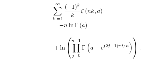
31: 25.11 Hurwitz Zeta Function

… ►

25.11.37

\sum_{k=1}^{\infty}\frac{(-1)^{k}}{k}\zeta\left(nk,a\right)=-n\ln\Gamma\left(a% \right)+\ln\left(\prod_{j=0}^{n-1}\Gamma\left(a-e^{(2j+1)\pi i/n}\right)\right),

n=2,3,4,\dots

\Re a\geq 1

ⓘ

Symbols:: $\Gamma\left(\NVar{z}\right)$ : gamma function, $\zeta\left(\NVar{s},\NVar{a}\right)$ : Hurwitz zeta function, $\pi$ : the ratio of the circumference of a circle to its diameter, $\mathrm{e}$ : base of natural logarithm, $\mathrm{i}$ : imaginary unit, $\ln\NVar{z}$ : principal branch of logarithm function, $\operatorname{ph}$ : phase, $\Re$ : real part, $k$ : nonnegative integer, $n$ : nonnegative integer and $a$ : real or complex parameter
Keywords:: infinite series, series representation
Source:: Adamchik and Srivastava (1998, (2.12), p. 136); with the choice $\operatorname{ph}\left(-1\right)=\pi$ , which is reasonable since the gamma function is single valued
Permalink:: http://dlmf.nist.gov/25.11.E37
Encodings:: pMML, png, TeX
See also:: Annotations for §25.11(xi), §25.11 and Ch.25

…

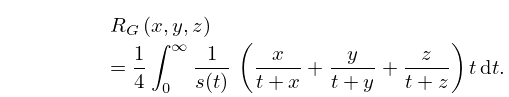
32: 19.16 Definitions

… ►

19.16.2_5

R_{G}\left(x,y,z\right)=\frac{1}{4}\int_{0}^{\infty}\frac{1}{s(t)}\*\left(% \frac{x}{t+x}+\frac{y}{t+y}+\frac{z}{t+z}\right)t\,\mathrm{d}t.

ⓘ

Defines:: $R_{G}\left(\NVar{x},\NVar{y},\NVar{z}\right)$ : symmetric elliptic integral of second kind
Symbols:: $\,\mathrm{d}\NVar{x}$ : differential of $x$ , $\int$ : integral and $s(t)$ : scaling factor
Source:: Carlson (1977b, (9.1-9))
Referenced by:: §19.16(i), §19.16(i), §19.21(ii), (19.23.7), (19.23.7), §19.23, Erratum (V1.1.0) for Rearrangement
Permalink:: http://dlmf.nist.gov/19.16.E2_5
Encodings:: pMML, png, TeX
Rearrangement (effective with 1.1.0):: This integral representation was moved from (19.23.7) and is taken as the definition of $R_{G}\left(x,y,z\right)$ . We have also employed the notation $s(t)$ for the factor of radicals.
See also:: Annotations for §19.16(i), §19.16 and Ch.19

… ►

19.16.7

\frac{3}{2}\int_{0}^{\infty}\frac{\,\mathrm{d}t}{\prod_{j=1}^{5}\sqrt{t+x_{j}}}.

ⓘ

Symbols:: $\,\mathrm{d}\NVar{x}$ : differential of $x$ and $\int$ : integral
Permalink:: http://dlmf.nist.gov/19.16.E7
Encodings:: pMML, png, TeX
See also:: Annotations for §19.16(i), §19.16 and Ch.19

►

§19.16(ii) $R_{-a}\left(\mathbf{b};\mathbf{z}\right)$

… ►

19.16.9

R_{-a}\left(\mathbf{b};\mathbf{z}\right)=\frac{1}{\mathrm{B}\left(a,a^{\prime}% \right)}\int_{0}^{\infty}t^{a^{\prime}-1}\prod^{n}_{j=1}(t+z_{j})^{-b_{j}}\,% \mathrm{d}t=\frac{1}{\mathrm{B}\left(a,a^{\prime}\right)}\int_{0}^{\infty}t^{a% -1}\prod^{n}_{j=1}(1+tz_{j})^{-b_{j}}\,\mathrm{d}t,

b_{1}+\cdots+b_{n}>a>0

b_{j}\in\mathbb{R}

z_{j}\in\mathbb{C}\setminus(-\infty,0]

ⓘ

Defines:: $R_{\NVar{-a}}\left(\NVar{b_{1}},\dots,\NVar{b_{n}};\NVar{z_{1}},\dots,\NVar{z_% {n}}\right)$ or $R_{\NVar{-a}}\left(\NVar{\mathbf{b}};\NVar{\mathbf{z}}\right)$ : multivariate hypergeometric function
Symbols:: $\mathrm{B}\left(\NVar{a},\NVar{b}\right)$ : beta function, $\mathbb{C}$ : complex plane, $\,\mathrm{d}\NVar{x}$ : differential of $x$ , $\in$ : element of, $\int$ : integral, $(\NVar{a},\NVar{b}]$ : half-closed interval, $\mathbb{R}$ : real line, $\setminus$ : set subtraction and $n$ : nonnegative integer
Referenced by:: §19.16(ii), §19.16(ii), §19.19, §19.20(iv), Erratum (V1.0.18) for Equation (19.16.9)
Permalink:: http://dlmf.nist.gov/19.16.E9
Encodings:: pMML, png, TeX
Clarification (effective with 1.0.18):: The constraint $a,a^{\prime}>0$ , was replaced with $b_{1}+\cdots+b_{n}>a>0$ , $b_{j}\in\mathbb{R}$ . It therefore follows from (19.16.10) that $a^{\prime}>0$ .
Suggested 2017-07-25 by Bastien Roucariès
See also:: Annotations for §19.16(ii), §19.16 and Ch.19

… ►For generalizations and further information, especially representation of the

R

-function as a Dirichlet average, see Carlson (1977b). …

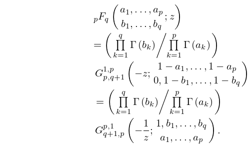
33: 16.18 Special Cases

… ►

16.18.1

{{}_{p}F_{q}}\left({a_{1},\dots,a_{p}\atop b_{1},\dots,b_{q}};z\right)=\left({% \textstyle\ifrac{\prod\limits_{k=1}^{q}\Gamma\left(b_{k}\right)}{\prod\limits_% {k=1}^{p}\Gamma\left(a_{k}\right)}}\right){G^{1,p}_{p,q+1}}\left(-z;{1-a_{1},% \dots,1-a_{p}\atop 0,1-b_{1},\dots,1-b_{q}}\right)=\left({\textstyle\ifrac{% \prod\limits_{k=1}^{q}\Gamma\left(b_{k}\right)}{\prod\limits_{k=1}^{p}\Gamma% \left(a_{k}\right)}}\right){G^{p,1}_{q+1,p}}\left(-\frac{1}{z};{1,b_{1},\dots,% b_{q}\atop a_{1},\dots,a_{p}}\right).

ⓘ

Symbols:: $\Gamma\left(\NVar{z}\right)$ : gamma function, ${{}_{\NVar{p}}F_{\NVar{q}}}\left(\NVar{a_{1},\dots,a_{p}};\NVar{b_{1},\dots,b_% {q}};\NVar{z}\right)$ or ${{}_{\NVar{p}}F_{\NVar{q}}}\left({\NVar{a_{1},\dots,a_{p}}\atop\NVar{b_{1},% \dots,b_{q}}};\NVar{z}\right)$ : alternatively ${{}_{\NVar{p}}F_{\NVar{q}}}\left(\NVar{\mathbf{a}};\NVar{\mathbf{b}};\NVar{z}\right)$ or ${{}_{\NVar{p}}F_{\NVar{q}}}\left({\NVar{\mathbf{a}}\atop\NVar{\mathbf{b}}};% \NVar{z}\right)$
generalized hypergeometric function, ${G^{\NVar{m},\NVar{n}}_{\NVar{p},\NVar{q}}}\left(\NVar{z};{\NVar{a_{1},\dots,a% _{p}}\atop\NVar{b_{1},\dots,b_{q}}}\right)$ or ${G^{\NVar{m},\NVar{n}}_{\NVar{p},\NVar{q}}}\left(\NVar{z};\NVar{\mathbf{a}};% \NVar{\mathbf{b}}\right)$ : Meijer $G$ -function, $p$ : nonnegative integer, $q$ : nonnegative integer, $z$ : complex variable, $a,a_{1},\ldots,a_{p}$ : real or complex parameters and $b,b_{1},\ldots,b_{q}$ : real or complex parameters
Permalink:: http://dlmf.nist.gov/16.18.E1
Encodings:: pMML, png, TeX
See also:: Annotations for §16.18 and Ch.16

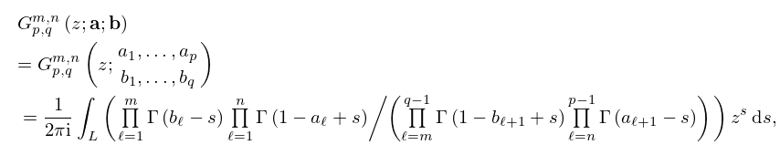
… ►Representations of special functions in terms of the Meijer

G

-function are given in Erdélyi et al. (1953a, §5.6), Luke (1969a, §§6.4–6.5), and Mathai (1993, §3.10). …

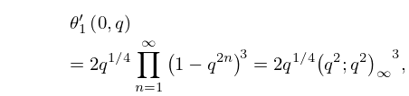
34: 20.4 Values at $z$ = 0

… ►

20.4.2

\theta_{1}'\left(0,q\right)=2q^{1/4}\prod\limits_{n=1}^{\infty}\left(1-q^{2n}% \right)^{3}=2q^{1/4}{\left(q^{2};q^{2}\right)_{\infty}}^{3},

ⓘ

Symbols:: $\theta_{\NVar{j}}\left(\NVar{z},\NVar{q}\right)$ : theta function, $\left(\NVar{a};\NVar{q}\right)_{\NVar{n}}$ : $q$ -Pochhammer symbol (or $q$ -shifted factorial), $n$ : integer and $q$ : nome
Referenced by:: Erratum (V1.0.28) for Equation (20.4.2)
Permalink:: http://dlmf.nist.gov/20.4.E2
Encodings:: pMML, png, TeX
Addition (effective with 1.0.28):: The representation in terms of ${\left(q^{2};q^{2}\right)_{\infty}}^{3}$ was added to this equation.
See also:: Annotations for §20.4(i), §20.4 and Ch.20

…

35: 1.18 Linear Second Order Differential Operators and Eigenfunction Expansions

… ►A complex linear vector space

V

is called an inner product space if an inner product

\left\langle u,v\right\rangle\in\mathbb{C}

is defined for all

u,v\in V

with the properties: (i)

\left\langle u,v\right\rangle

is complex linear in

u

; (ii)

\left\langle u,v\right\rangle=\overline{\left\langle v,u\right\rangle}

; (iii)

\left\langle v,v\right\rangle\geq 0

; (iv) if

\left\langle v,v\right\rangle=0

then

v=0

. With norm defined by …Two elements

u

and

v

V

are orthogonal if

\left\langle u,v\right\rangle=0

. … ►thus generalizing the inner product of (1.18.9). … ►The adjoint

{T}^{*}

T

does satisfy

\left\langle Tf,g\right\rangle=\left\langle f,{T}^{*}g\right\rangle

where

\left\langle f,g\right\rangle=\int_{a}^{b}f(x)g(x)\,\mathrm{d}x

. …

36: 15.17 Mathematical Applications

… ►

§15.17(iii) Group Representations

… ►In combinatorics, hypergeometric identities classify single sums of products of binomial coefficients. …

37: 16.5 Integral Representations and Integrals

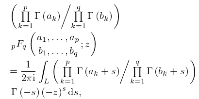
§16.5 Integral Representations and Integrals

… ►

16.5.1

\left({\textstyle\ifrac{\prod\limits_{k=1}^{p}\Gamma\left(a_{k}\right)}{\prod% \limits_{k=1}^{q}\Gamma\left(b_{k}\right)}}\right){{}_{p}F_{q}}\left({a_{1},% \dots,a_{p}\atop b_{1},\dots,b_{q}};z\right)=\frac{1}{2\pi\mathrm{i}}\int_{L}% \left({\textstyle\ifrac{\prod\limits_{k=1}^{p}\Gamma\left(a_{k}+s\right)}{% \prod\limits_{k=1}^{q}\Gamma\left(b_{k}+s\right)}}\right)\Gamma\left(-s\right)% (-z)^{s}\,\mathrm{d}s,

ⓘ

Symbols:: $\Gamma\left(\NVar{z}\right)$ : gamma function, ${{}_{\NVar{p}}F_{\NVar{q}}}\left(\NVar{a_{1},\dots,a_{p}};\NVar{b_{1},\dots,b_% {q}};\NVar{z}\right)$ or ${{}_{\NVar{p}}F_{\NVar{q}}}\left({\NVar{a_{1},\dots,a_{p}}\atop\NVar{b_{1},% \dots,b_{q}}};\NVar{z}\right)$ : alternatively ${{}_{\NVar{p}}F_{\NVar{q}}}\left(\NVar{\mathbf{a}};\NVar{\mathbf{b}};\NVar{z}\right)$ or ${{}_{\NVar{p}}F_{\NVar{q}}}\left({\NVar{\mathbf{a}}\atop\NVar{\mathbf{b}}};% \NVar{z}\right)$
generalized hypergeometric function, $\pi$ : the ratio of the circumference of a circle to its diameter, $\,\mathrm{d}\NVar{x}$ : differential of $x$ , $\mathrm{i}$ : imaginary unit, $\int$ : integral, $p$ : nonnegative integer, $q$ : nonnegative integer, $z$ : complex variable, $a,a_{1},\ldots,a_{p}$ : real or complex parameters and $b,b_{1},\ldots,b_{q}$ : real or complex parameters
Referenced by:: §13.6(vi), §16.11(i), §16.5, §16.5
Permalink:: http://dlmf.nist.gov/16.5.E1
Encodings:: pMML, png, TeX
See also:: Annotations for §16.5 and Ch.16

… ►Then the integral converges when

p<q+1

provided that

z\neq 0

, or when

p=q+1

provided that

0<|z|<1

, and provides an integral representation of the left-hand side with these conditions. … ►In the case

p=q

the left-hand side of (16.5.1) is an entire function, and the right-hand side supplies an integral representation valid when

|\operatorname{ph}\left(-z\right)|<\pi/2

. … ►For further integral representations and integrals see Apelblat (1983, §16), Erdélyi et al. (1953a, §4.6), Erdélyi et al. (1954a, §§6.9 and 7.5), Luke (1969a, §3.6), and Prudnikov et al. (1990, §§2.22, 4.2.4, and 4.3.1). …

38: Bibliography

… ►

T. Agoh and K. Dilcher (2011) Integrals of products of Bernoulli polynomials. J. Math. Anal. Appl. 381 (1), pp. 10–16.

ⓘ

External Links:: ISSN 0022-247X, Document, FullText, MathReview (Pablo Manuel Román), ZentralBlatt
Referenced by:: §24.13(i), §24.13(i).
Encodings:: BibTeX

… ►

J. R. Albright (1977) Integrals of products of Airy functions. J. Phys. A 10 (4), pp. 485–490.

ⓘ

External Links:: Document, MathReview (Y. L. Luke), ZentralBlatt
Referenced by:: (9.11.10), (9.11.5), (9.11.6), (9.11.7), (9.11.8), (9.11.9), §9.11(iv), §9.11(iv).
Encodings:: BibTeX

… ►

A. Apelblat (1991) Integral representation of Kelvin functions and their derivatives with respect to the order. Z. Angew. Math. Phys. 42 (5), pp. 708–714.

ⓘ

External Links:: ISSN 0044-2275, Document, MathReview (A. de Castro Brzezicki), ZentralBlatt
Referenced by:: §10.61(v), §10.64.
Encodings:: BibTeX

… ►

R. Askey and J. Fitch (1969) Integral representations for Jacobi polynomials and some applications. J. Math. Anal. Appl. 26 (2), pp. 411–437.

ⓘ

External Links:: Document, MathReview (D. L. Colton), ZentralBlatt
Referenced by:: §18.17(iv).
Encodings:: BibTeX

… ►

R. Askey (1974) Jacobi polynomials. I. New proofs of Koornwinder’s Laplace type integral representation and Bateman’s bilinear sum. SIAM J. Math. Anal. 5, pp. 119–124.

ⓘ

External Links:: ISSN 1095-7154, Document, MathReview (R. P. Soni), ZentralBlatt
Referenced by:: §18.18(iv).
Encodings:: BibTeX

…

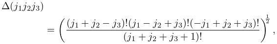
39: 34.2 Definition: $\mathit{3j}$ Symbol

… ►See Figure 34.2.1 for a schematic representation. … ►

34.2.4

\begin{pmatrix}j_{1}&j_{2}&j_{3}\\ m_{1}&m_{2}&m_{3}\end{pmatrix}={(-1)^{j_{1}-j_{2}-m_{3}}}\Delta(j_{1}j_{2}j_{3% })\left((j_{1}+m_{1})!(j_{1}-m_{1})!(j_{2}+m_{2})!(j_{2}-m_{2})!(j_{3}+m_{3})!% (j_{3}-m_{3})!\right)^{\frac{1}{2}}\*\sum_{s}\frac{(-1)^{s}}{s!(j_{1}+j_{2}-j_% {3}-s)!(j_{1}-m_{1}-s)!(j_{2}+m_{2}-s)!(j_{3}-j_{2}+m_{1}+s)!(j_{3}-j_{1}-m_{2% }+s)!},

ⓘ

Defines:: $\begin{pmatrix}\NVar{j_{1}}&\NVar{j_{2}}&\NVar{j_{3}}\\ \NVar{m_{1}}&\NVar{m_{2}}&\NVar{m_{3}}\end{pmatrix}$ : $\mathit{3j}$ symbol
Symbols:: $!$ : factorial (as in $n!$ ), $j,j_{r}$ : non-negative integers or non-negative integers plus one half., $\Delta(j_{1}j_{2}j_{3})$ : product and $s$ : nonnegative integer
Permalink:: http://dlmf.nist.gov/34.2.E4
Encodings:: pMML, png, TeX
See also:: Annotations for §34.2 and Ch.34

… ►

34.2.5

\Delta(j_{1}j_{2}j_{3})=\left(\frac{(j_{1}+j_{2}-j_{3})!(j_{1}-j_{2}+j_{3})!(-% j_{1}+j_{2}+j_{3})!}{(j_{1}+j_{2}+j_{3}+1)!}\right)^{\frac{1}{2}},

ⓘ

Defines:: $\Delta(j_{1}j_{2}j_{3})$ : product (locally)
Symbols:: $!$ : factorial (as in $n!$ ) and $j,j_{r}$ : non-negative integers or non-negative integers plus one half.
Permalink:: http://dlmf.nist.gov/34.2.E5
Encodings:: pMML, png, TeX
See also:: Annotations for §34.2 and Ch.34

… ►

34.2.6

\begin{pmatrix}j_{1}&j_{2}&j_{3}\\ m_{1}&m_{2}&m_{3}\end{pmatrix}={(-1)^{j_{2}-m_{1}+m_{3}}}\frac{(j_{1}+j_{2}+m_% {3})!(j_{2}+j_{3}-m_{1})!}{\Delta(j_{1}j_{2}j_{3})(j_{1}+j_{2}+j_{3}+1)!}\left% (\frac{(j_{1}+m_{1})!(j_{3}-m_{3})!}{(j_{1}-m_{1})!(j_{2}+m_{2})!(j_{2}-m_{2})% !(j_{3}+m_{3})!}\right)^{\frac{1}{2}}\*{{{}_{3}F_{2}}\left(-j_{1}-j_{2}-j_{3}-% 1,-j_{1}+m_{1},-j_{3}-m_{3};-j_{1}-j_{2}-m_{3},-j_{2}-j_{3}+m_{1};1\right)},

ⓘ

Symbols:: ${{}_{\NVar{p}}F_{\NVar{q}}}\left(\NVar{a_{1},\dots,a_{p}};\NVar{b_{1},\dots,b_% {q}};\NVar{z}\right)$ or ${{}_{\NVar{p}}F_{\NVar{q}}}\left({\NVar{a_{1},\dots,a_{p}}\atop\NVar{b_{1},% \dots,b_{q}}};\NVar{z}\right)$ : alternatively ${{}_{\NVar{p}}F_{\NVar{q}}}\left(\NVar{\mathbf{a}};\NVar{\mathbf{b}};\NVar{z}\right)$ or ${{}_{\NVar{p}}F_{\NVar{q}}}\left({\NVar{\mathbf{a}}\atop\NVar{\mathbf{b}}};% \NVar{z}\right)$
generalized hypergeometric function, $!$ : factorial (as in $n!$ ), $\begin{pmatrix}\NVar{j_{1}}&\NVar{j_{2}}&\NVar{j_{3}}\\ \NVar{m_{1}}&\NVar{m_{2}}&\NVar{m_{3}}\end{pmatrix}$ : $\mathit{3j}$ symbol, $j,j_{r}$ : non-negative integers or non-negative integers plus one half. and $\Delta(j_{1}j_{2}j_{3})$ : product
Referenced by:: §18.38(iii)
Permalink:: http://dlmf.nist.gov/34.2.E6
Encodings:: pMML, png, TeX
See also:: Annotations for §34.2 and Ch.34

►where

{{}_{3}F_{2}}

is defined as in §16.2. …

40: 16.17 Definition

… ►Then the Meijer $G$ -function is defined via the Mellin–Barnes integral representation: ►

16.17.1

{G^{m,n}_{p,q}}\left(z;\mathbf{a};\mathbf{b}\right)={G^{m,n}_{p,q}}\left(z;{a_% {1},\dots,a_{p}\atop b_{1},\dots,b_{q}}\right)=\frac{1}{2\pi\mathrm{i}}\int_{L% }\left({\textstyle\ifrac{\prod\limits_{\ell=1}^{m}\Gamma\left(b_{\ell}-s\right% )\prod\limits_{\ell=1}^{n}\Gamma\left(1-a_{\ell}+s\right)}{\left(\prod\limits_% {\ell=m}^{q-1}\Gamma\left(1-b_{\ell+1}+s\right)\prod\limits_{\ell=n}^{p-1}% \Gamma\left(a_{\ell+1}-s\right)\right)}}\right)z^{s}\,\mathrm{d}s,

ⓘ

Defines:: ${G^{\NVar{m},\NVar{n}}_{\NVar{p},\NVar{q}}}\left(\NVar{z};{\NVar{a_{1},\dots,a% _{p}}\atop\NVar{b_{1},\dots,b_{q}}}\right)$ or ${G^{\NVar{m},\NVar{n}}_{\NVar{p},\NVar{q}}}\left(\NVar{z};\NVar{\mathbf{a}};% \NVar{\mathbf{b}}\right)$ : Meijer $G$ -function
Symbols:: $\Gamma\left(\NVar{z}\right)$ : gamma function, $\pi$ : the ratio of the circumference of a circle to its diameter, $\,\mathrm{d}\NVar{x}$ : differential of $x$ , $\mathrm{i}$ : imaginary unit, $\int$ : integral, $p$ : nonnegative integer, $q$ : nonnegative integer, $z$ : complex variable, $a,a_{1},\ldots,a_{p}$ : real or complex parameters and $b,b_{1},\ldots,b_{q}$ : real or complex parameters
Referenced by:: Figure 16.17.1, Figure 16.17.1, §16.19
Permalink:: http://dlmf.nist.gov/16.17.E1
Encodings:: pMML, png, TeX
See also:: Annotations for §16.17 and Ch.16

… ►

…

Figure 16.17.1: s-plane. Path

L

for the integral representation (16.17.1) of the Meijer

G

-function.

… ►

16.17.3

A_{p,q,k}^{m,n}(z)=\ifrac{\prod\limits_{\begin{subarray}{c}\ell=1\\ \ell\neq k\end{subarray}}^{m}\Gamma\left(b_{\ell}-b_{k}\right)\prod\limits_{% \ell=1}^{n}\Gamma\left(1+b_{k}-a_{\ell}\right)z^{b_{k}}}{\left(\prod\limits_{% \ell=m}^{q-1}\Gamma\left(1+b_{k}-b_{\ell+1}\right)\prod\limits_{\ell=n}^{p-1}% \Gamma\left(a_{\ell+1}-b_{k}\right)\right)}.

ⓘ

Defines:: $A_{p,q}^{m,n}(z)$ : coefficient (locally)
Symbols:: $\Gamma\left(\NVar{z}\right)$ : gamma function, $p$ : nonnegative integer, $q$ : nonnegative integer, $z$ : complex variable, $a,a_{1},\ldots,a_{p}$ : real or complex parameters and $b,b_{1},\ldots,b_{q}$ : real or complex parameters
Permalink:: http://dlmf.nist.gov/16.17.E3
Encodings:: pMML, png, TeX
See also:: Annotations for §16.17 and Ch.16