of%20one%20variable

SearchAdvancedHelp

(0.002 seconds)

21—30 of 30 matching pages

21: Bibliography L

… ►

The solutions of the Mathieu equation with a complex variable and at least one parameter large. Trans. Amer. Math. Soc. 36 (3), pp. 637–695.

ⓘ

External Links:

ISSN 0002-9947, FullText, MathReview Entry, ZentralBlatt

Referenced by:

§28.8(iv).

Encodings:

BibTeX

… ►

Algorithm 917: complex double-precision evaluation of the Wright $\omega$ function. ACM Trans. Math. Software 38 (3), pp. Art. 20, 17.

ⓘ

External Links:

ISSN 0098-3500, Document, FullText, MathReview Entry, ZentralBlatt

Referenced by:

§4.13, 2nd item, §4.48(iv).

Encodings:

BibTeX

… ►

An asymptotic estimate for the Bernoulli and Euler numbers. Canad. Math. Bull. 20 (1), pp. 109–111.

ⓘ

External Links:

MathReview (D. H. Lehmer), ZentralBlatt

Referenced by:

§24.11.

Encodings:

BibTeX

… ►

On the maxima and minima of Bernoulli polynomials. Amer. Math. Monthly 47 (8), pp. 533–538.

ⓘ

External Links:

FullText, MathReview (W. E. Milne), ZentralBlatt

Referenced by:

§24.12(i), §24.9.

Encodings:

BibTeX

… ►

More than one third of zeros of Riemann’s zeta-function are on $\sigma =\frac{1}{2}$ . Advances in Math. 13 (4), pp. 383–436.

ⓘ

External Links:

Document, MathReview (H. L. Montgomery), ZentralBlatt

Referenced by:

§25.10(ii), Erratum (V1.1.4) for Subsection 25.10(ii).

Encodings:

BibTeX

…

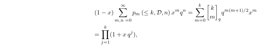
22: 26.10 Integer Partitions: Other Restrictions

… ►If more than one restriction applies, then the restrictions are separated by commas, for example, $p(𝒟2,\in T,n)$. … ►

Table 26.10.1: Partitions restricted by difference conditions, or equivalently with parts from $A_{j,k}$.

► ►►►

	$p(𝒟,n)$	$p(𝒟2,n)$	$p(𝒟2,\in T,n)$	$p({𝒟}^{\prime }3,n)$
…
$20$	$64$	$31$	$20$	$18$

►

… ►

26.10.3 $$(1-x)\sum _{m,n=0}^{\mathrm{\infty }}{p}_m(\le k,𝒟,n)x^m{q}^n=\sum _{m=0}^k{\left[\genfrac{}{}{0.0pt}{}{k}{m}\right]}_q{q}^{m(m+1)/2}{x}^m=\prod _{j=1}^k(1+x{q}^j),$$ ,

ⓘ

Symbols:

${\left[\genfrac{}{}{0.0pt}{}{n}{m}\right]}_q$: $q$-binomial coefficient (or Gaussian polynomial), $p_k(\le m,n)$: number of partitions of $n$ into at most $k$ parts, each less than or equal to $m$ , $x$: real variable, $j$: nonnegative integer, $k$: nonnegative integer, $m$: nonnegative integer, $n$: nonnegative integer and $q$: parameter

Referenced by:

§26.10(ii)

Permalink:

http://dlmf.nist.gov/26.10.E3

Encodings:

pMML, png, TeX

See also:

Annotations for §26.10(ii), §26.10 and Ch.26

… ►

26.10.20

ⓘ

Symbols:

$\in$: element of, $\lfloor x\rfloor$: floor of $x$ , $\mathbb{Z}$: set of all integers, $\notin$: not an element of and $x$: real variable

Permalink:

http://dlmf.nist.gov/26.10.E20

Encodings:

pMML, png, TeX

See also:

Annotations for §26.10(vi), §26.10 and Ch.26

…

23: Bibliography B

… ►

Pionic atoms. Annual Review of Nuclear and Particle Science 20, pp. 467–508.

ⓘ

External Links:

Document

Referenced by:

§33.22(iv).

Encodings:

BibTeX

… ►

A program for computing the Riemann zeta function for complex argument. Comput. Phys. Comm. 20 (3), pp. 441–445.

ⓘ

Notes:

Double-precision Fortran, maximum accuracy 10S.

External Links:

Document, Code, ZentralBlatt

Referenced by:

1st item.

Encodings:

BibTeX

… ►

Coulomb functions (negative energies). Comput. Phys. Comm. 20 (3), pp. 447–458.

ⓘ

Notes:

Double-precision Fortran code.

External Links:

Document, Code

Referenced by:

1st item, 4th item.

Encodings:

BibTeX

… ►

Some solutions of the problem of forced convection. Philos. Mag. Series 7 20, pp. 322–343.

ⓘ

External Links:

Document, ZentralBlatt

Referenced by:

§10.73(iv).

Encodings:

BibTeX

… ►

Bessel functions and modular relations of higher type and hyperbolic differential equations. Comm. Sém. Math. Univ. Lund [Medd. Lunds Univ. Mat. Sem.] 1952 (Tome Supplementaire), pp. 12–20.

ⓘ

External Links:

MathReview (S. C. van Veen), ZentralBlatt

Referenced by:

§35.5(i).

Encodings:

BibTeX

…

24: 12.11 Zeros

… ►For further information on these cases see Dean (1966). … ►

§12.11(ii) Asymptotic Expansions of Large Zeros

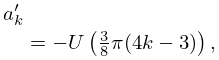
… ►Numerical calculations in this case show that $z_{\frac{1}{2},s}$ corresponds to the $s$th zero on the string; compare §7.13(ii). … ►

12.11.8 $$q_0(\zeta )=t(\zeta ).$$

ⓘ

Symbols:

$\zeta$: change of variable

Permalink:

http://dlmf.nist.gov/12.11.E8

Encodings:

pMML, png, TeX

See also:

Annotations for §12.11(iii), §12.11 and Ch.12

… ►

12.11.9 $$u_{a,1}\sim 2^{\frac{1}{2}}\mu \left(1-\mathrm{1.85575\hspace{0.33em}708}{\mu }^{-4/3}-\mathrm{0.34438\hspace{0.33em}34}{\mu }^{-8/3}-\mathrm{0.16871\hspace{0.33em}5}{\mu }^{-4}-0.11414{\mu }^{-16/3}-0.0808{\mu }^{-20/3}-\mathrm{\cdots }\right),$$

ⓘ

Symbols:

$\sim$: Poincaré asymptotic expansion, $a$: real or complex parameter and $u_{a,s}$: zeros

Referenced by:

§12.11(iii)

Permalink:

http://dlmf.nist.gov/12.11.E9

Encodings:

pMML, png, TeX

See also:

Annotations for §12.11(iii), §12.11 and Ch.12

…

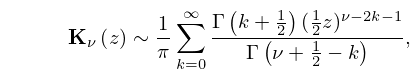
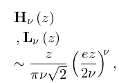
25: 30.9 Asymptotic Approximations and Expansions

… ►

$$2^{20}{\beta }_5=-527q^7-61529q^5-\mathrm{10\hspace{0.33em}43961}{q}^3-\mathrm{22\hspace{0.33em}41599}q+32m^2(5739q^5+\mathrm{1\hspace{0.33em}27550}{q}^3+\mathrm{2\hspace{0.33em}98951}q)-2048m^4(355q^3+1505q)+65536m^{6}q.$$

… ►For uniform asymptotic expansions in terms of Airy or Bessel functions for real values of the parameters, complex values of the variable, and with explicit error bounds see Dunster (1986). … ►For uniform asymptotic expansions in terms of elementary, Airy, or Bessel functions for real values of the parameters, complex values of the variable, and with explicit error bounds see Dunster (1992, 1995). … ►The asymptotic behavior of ${\mathrm{𝖯𝗌}}_n^m(x,{\gamma }^2)$ and ${\mathrm{𝖰𝗌}}_n^m(x,{\gamma }^2)$ as $x\to \pm 1$ is given in Erdélyi et al. (1955, p. 151). …

26: Bibliography I

… ►

The real roots of Bernoulli polynomials. Ann. Univ. Turku. Ser. A I 37, pp. 1–20.

ⓘ

External Links:

MathReview (D. H. Lehmer), ZentralBlatt

Referenced by:

§24.12(i).

Encodings:

BibTeX

… ►

On polynomials orthogonal with respect to certain Sobolev inner products. J. Approx. Theory 65 (2), pp. 151–175.

ⓘ

External Links:

ISSN 0021-9045, Document, MathReview (R. A. Askey), ZentralBlatt

Referenced by:

§18.36(ii).

Encodings:

BibTeX

… ►

More on electrostatic models for zeros of orthogonal polynomials. Numer. Funct. Anal. Optim. 21 (1-2), pp. 191–204.

ⓘ

External Links:

ISSN 0163-0563, FullText, MathReview (M. E. Muldoon), ZentralBlatt

Referenced by:

§18.39(v).

Encodings:

BibTeX

►

Classical and Quantum Orthogonal Polynomials in One Variable. Encyclopedia of Mathematics and its Applications, Vol. 98, Cambridge University Press, Cambridge.

ⓘ

External Links:

ISBN 978-0-521-78201-2; 0-521-78201-5, MathReview Entry, ZentralBlatt

Referenced by:

§1.4(v), Profile Mourad E.H. Ismail, Erratum (V1.0.20) for Chapter 18 Orthogonal Polynomials.

Encodings:

BibTeX

►

Classical and Quantum Orthogonal Polynomials in One Variable. Encyclopedia of Mathematics and its Applications, Vol. 98, Cambridge University Press, Cambridge.

ⓘ

Notes:

With two chapters by Walter Van Assche, With a foreword by Richard A. Askey, Corrected reprint of the 2005 original.

External Links:

ISBN 978-0-521-14347-9, MathReview Entry, ZentralBlatt

Referenced by:

§18.12, (18.15.4_5), (18.16.19), (18.16.20), (18.16.21), §18.17(ii), §18.18(vii), §18.19, (18.2.20), §18.2(vi), §18.2(xii), §18.2(xii), §18.2(x), §18.20(i), §18.20(ii), §18.21(ii), §18.22(i), §18.22(ii), §18.22(iii), §18.23, §18.25(i), §18.25(iii), §18.26(i), §18.26(iv), (18.27.4), §18.27(i), §18.27(ii), §18.27(iii), §18.27(v), §18.27(vi), §18.28(i), §18.28(ii), §18.28(iii), §18.28(v), §18.28(vi), §18.28(vii), §18.28(viii), §18.30(vi), §18.30(vii), §18.30(iii), §18.30(iv), §18.30, §18.30(vi), §18.34(i), §18.34(ii), §18.34(ii), §18.34(iii), (18.35.4), (18.35.5), (18.35.6), (18.35.6_2), (18.35.6_3), (18.35.6_4), (18.35.7), (18.35.8), §18.35(ii), §18.35(iii), §18.36(iii), §18.38(ii), §18.39(iv), §18.39(iv), §18.39(iv), (18.40.4), Profile Mourad E.H. Ismail, Erratum (V1.0.20) for Chapter 18 Orthogonal Polynomials.

Encodings:

BibTeX

…

27: 11.6 Asymptotic Expansions

… ►

11.6.1 $${𝐊}_{\nu }\left(z\right)\sim \frac{1}{\pi }\sum _{k=0}^{\mathrm{\infty }}\frac{\mathrm{\Gamma }\left(k+\frac{1}{2}\right){(\frac{1}{2}z)}^{\nu -2k-1}}{\mathrm{\Gamma }\left(\nu +\frac{1}{2}-k\right)},$$ $|\mathrm{ph}z|\le \pi -\delta$,

ⓘ

Symbols:

$\mathrm{\Gamma }\left(z\right)$: gamma function, ${𝐊}_{\nu }\left(z\right)$: Struve function, $\sim$: Poincaré asymptotic expansion, $\pi$: the ratio of the circumference of a circle to its diameter, $\mathrm{ph}$: phase, $z$: complex variable, $\nu$: real or complex order, $k$: nonnegative integer and $\delta$: arbitrary small positive constant

A&S Ref:

12.1.29

Referenced by:

§11.6(i), §11.6(i), §11.6(i), §11.6(i)

Permalink:

http://dlmf.nist.gov/11.6.E1

Encodings:

pMML, png, TeX

See also:

Annotations for §11.6(i), §11.6 and Ch.11

… ►If the series on the right-hand side of (11.6.1) is truncated after $m(\ge 0)$ terms, then the remainder term $R_m(z)$ is $O\left(z^{\nu -2m-1}\right)$. … ►

11.6.2 $${𝐌}_{\nu }\left(z\right)\sim \frac{1}{\pi }\sum _{k=0}^{\mathrm{\infty }}{(-1)}^{k+1}\frac{\mathrm{\Gamma }\left(k+\frac{1}{2}\right){(\frac{1}{2}z)}^{\nu -2k-1}}{\mathrm{\Gamma }\left(\nu +\frac{1}{2}-k\right)},$$ $|\mathrm{ph}z|\le \frac{1}{2}\pi -\delta$.

ⓘ

Symbols:

$\mathrm{\Gamma }\left(z\right)$: gamma function, ${𝐌}_{\nu }\left(z\right)$: modified Struve function, $\sim$: Poincaré asymptotic expansion, $\pi$: the ratio of the circumference of a circle to its diameter, $\mathrm{ph}$: phase, $z$: complex variable, $\nu$: real or complex order, $k$: nonnegative integer and $\delta$: arbitrary small positive constant

A&S Ref:

12.2.6

Referenced by:

§11.6(i), §11.6(i), §11.6(i)

Permalink:

http://dlmf.nist.gov/11.6.E2

Encodings:

pMML, png, TeX

See also:

Annotations for §11.6(i), §11.6 and Ch.11

… ►

11.6.5 $${𝐇}_{\nu }\left(z\right),{𝐋}_{\nu }\left(z\right)\sim \frac{z}{\pi \nu \sqrt{2}}{\left(\frac{\mathrm{e}z}{2\nu }\right)}^{\nu },$$ $|\mathrm{ph}\nu |\le \pi -\delta$.

ⓘ

Symbols:

${𝐇}_{\nu }\left(z\right)$: Struve function, $\sim$: asymptotic equality, $\pi$: the ratio of the circumference of a circle to its diameter, $\mathrm{e}$: base of natural logarithm, ${𝐋}_{\nu }\left(z\right)$: modified Struve function, $\mathrm{ph}$: phase, $z$: complex variable, $\nu$: real or complex order and $\delta$: arbitrary small positive constant

Referenced by:

(11.11.7)

Permalink:

http://dlmf.nist.gov/11.6.E5

Encodings:

pMML, png, TeX

See also:

Annotations for §11.6(ii), §11.6 and Ch.11

… ►

$c_3(\lambda )=20{\lambda }^{-6}-4{\lambda }^{-4},$

…

28: Bibliography S

… ►

Transformations of the Jacobian amplitude function and its calculation via the arithmetic-geometric mean. SIAM J. Math. Anal. 20 (6), pp. 1514–1528.

ⓘ

External Links:

ISSN 0036-1410, Document, MathReview (J. M. H. Peters), ZentralBlatt

Referenced by:

§22.19(i), §22.20(vi).

Encodings:

BibTeX

… ►

Uniform asymptotic forms of modified Mathieu functions. Quart. J. Mech. Appl. Math. 20 (3), pp. 365–380.

ⓘ

External Links:

Document, MathReview (F. W. J. Olver), ZentralBlatt

Referenced by:

§28.8(iv).

Encodings:

BibTeX

… ►

Text-book on Spherical Astronomy. Fifth edition, Cambridge University Press, Cambridge.

ⓘ

External Links:

MathReview

Referenced by:

§4.42(iii).

Encodings:

BibTeX

… ►

A Maple package for symmetric functions. J. Symbolic Comput. 20 (5-6), pp. 755–768.

ⓘ

Notes:

For software see John Stembridge’s home page. The SF package contains Maple software for zonal, Jack, and Macdonald polynomials.

External Links:

Home Page, ISSN 0747-7171, Document, MathReview, ZentralBlatt

Referenced by:

3rd item.

Encodings:

BibTeX

… ►

Numerical Methods Based on Sinc and Analytic Functions. Springer Series in Computational Mathematics, Vol. 20, Springer-Verlag, New York.

ⓘ

Notes:

Sinc-Pack, a set of 480 Matlab programs with a 470-page tutorial, is available for purchase from SINC, LLC by contacting Frank Stenger.

External Links:

ISBN 0-387-94008-1, MathReview (B. Boyanov), ZentralBlatt

Referenced by:

§3.3(vi), §3.4(i), §3.5(i).

Encodings:

BibTeX

…

29: 9.9 Zeros

… ►On the real line, $\mathrm{Ai}\left(x\right)$, ${\mathrm{Ai}}^{\prime }\left(x\right)$, $\mathrm{Bi}\left(x\right)$, ${\mathrm{Bi}}^{\prime }\left(x\right)$ each have an infinite number of zeros, all of which are negative. … ►If $k$ is regarded as a continuous variable, then … ►

9.9.6 $$a_k=-T\left(\frac{3}{8}\pi (4k-1)\right),$$

ⓘ

Symbols:

$\pi$: the ratio of the circumference of a circle to its diameter, $a_k$: $k$th zero of Airy $\mathrm{Ai}$ , $k$: nonnegative integer and $T$: expansion

Source:

Olver (1954, (A 20))

Permalink:

http://dlmf.nist.gov/9.9.E6

Encodings:

pMML, png, TeX

See also:

Annotations for §9.9(iv), §9.9 and Ch.9

►

9.9.7 $${\mathrm{Ai}}^{\prime }\left(a_k\right)={(-1)}^{k-1}V\left(\frac{3}{8}\pi (4k-1)\right),$$

ⓘ

Symbols:

$\mathrm{Ai}\left(z\right)$: Airy function, $\pi$: the ratio of the circumference of a circle to its diameter, $a_k$: $k$th zero of Airy $\mathrm{Ai}$ , $k$: nonnegative integer and $V$: expansion

Source:

Olver (1954, (A 20))

Permalink:

http://dlmf.nist.gov/9.9.E7

Encodings:

pMML, png, TeX

See also:

Annotations for §9.9(iv), §9.9 and Ch.9

►

9.9.8 $$a_k^{\prime }=-U\left(\frac{3}{8}\pi (4k-3)\right),$$

ⓘ

Symbols:

$\pi$: the ratio of the circumference of a circle to its diameter, $a_k^{\prime }$: $k$th zero of Airy ${\mathrm{Ai}}^{\prime }$ , $k$: nonnegative integer and $U$: expansion

Source:

Olver (1954, (A 20))

Permalink:

http://dlmf.nist.gov/9.9.E8

Encodings:

pMML, png, TeX

See also:

Annotations for §9.9(iv), §9.9 and Ch.9

…

30: 8.17 Incomplete Beta Functions

… ►Throughout §§8.17 and 8.18 we assume that $a>0$, $b>0$, and $0\le x\le 1$. … ►

8.17.4 $$I_x(a,b)=1-I_{1-x}(b,a).$$

ⓘ

Symbols:

$I_x(a,b)$: incomplete beta function, $a$: parameter, $b$: parameter and $x$: variable

A&S Ref:

6.6.3 (Symmetry relation)

Referenced by:

§8.17(v), §8.18(i)

Permalink:

http://dlmf.nist.gov/8.17.E4

Encodings:

pMML, png, TeX

See also:

Annotations for §8.17(i), §8.17 and Ch.8

… ►With $a>0$, $b>0$, and , …where and the branches of $s^{-a}$ and ${(1-s)}^{-b}$ are continuous on the path and assume their principal values when $s=c$. … ►

8.17.24 $$I_x(m,n)={(1-x)}^n\sum _{j=m}^{\mathrm{\infty }}\left(\genfrac{}{}{0.0pt}{}{n+j-1}{j}\right)x^j,$$ $m,n$ positive integers; .

ⓘ

Symbols:

$I_x(a,b)$: incomplete beta function, $\left(\genfrac{}{}{0.0pt}{}{m}{n}\right)$: binomial coefficient, $n$: nonnegative integer and $x$: variable

A&S Ref:

26.5.26 (The upper limit of summation has been corrected.)

Referenced by:

§8.17(i), Erratum (V1.0.5) for Chapters 8, 20, 36

Permalink:

http://dlmf.nist.gov/8.17.E24

Encodings:

pMML, png, TeX

Addition (effective with 1.0.5):

This equation is the same as Equation (26.5.26) of Abramowitz and Stegun (1964), except that the upper limit of the summation has been corrected to $\mathrm{\infty }$.

Suggested 2011-03-23 by Stephen Bourn

See also:

Annotations for §8.17(vii), §8.17 and Ch.8

…