of%20arbitrary%20order
♦
8 matching pages ♦
(0.003 seconds)
8 matching pages
1: 11.6 Asymptotic Expansions
…
►where is an arbitrary small positive constant.
…
►
…
►
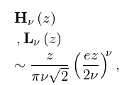
§11.6(ii) Large , Fixed
►
11.6.5
.
…
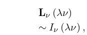
►
11.6.9
,
…
2: Bibliography O
…
►
Hyperasymptotic solutions of second-order linear differential equations. I.
Methods Appl. Anal. 2 (2), pp. 173–197.
…
►
An error analysis of the modified Clenshaw method for evaluating Chebyshev and Fourier series.
J. Inst. Math. Appl. 20 (3), pp. 379–391.
…
►
Error bounds for asymptotic solutions of second-order differential equations having an irregular singularity of arbitrary rank.
J. Soc. Indust. Appl. Math. Ser. B Numer. Anal. 2 (2), pp. 244–249.
…
►
Connection formulas for second-order differential equations having an arbitrary number of turning points of arbitrary multiplicities.
SIAM J. Math. Anal. 8 (4), pp. 673–700.
►
Second-order differential equations with fractional transition points.
Trans. Amer. Math. Soc. 226, pp. 227–241.
…
3: Bibliography S
…
►
Arbitrary
symbols for
.
Comput. Phys. Comm. 1 (3), pp. 207–215.
…
►
Uniform asymptotic forms of modified Mathieu functions.
Quart. J. Mech. Appl. Math. 20 (3), pp. 365–380.
…
►
Computation of infinite integrals involving Bessel functions of arbitrary order by the -transformation.
J. Comput. Appl. Math. 78 (1), pp. 125–130.
…
►
Euler-Maclaurin expansions for integrals with arbitrary algebraic endpoint singularities.
Math. Comp. 81 (280), pp. 2159–2173.
►
Euler-Maclaurin expansions for integrals with arbitrary algebraic-logarithmic endpoint singularities.
Constr. Approx. 36 (3), pp. 331–352.
…
4: 18.39 Applications in the Physical Sciences
…
►The nature of, and notations and common vocabulary for, the eigenvalues and eigenfunctions of self-adjoint second order differential operators is overviewed in §1.18.
…
►The fundamental quantum Schrödinger operator, also called the Hamiltonian, , is a second order differential operator of the form
…
►If is an arbitrary unit normalized function in the domain of then, by self-adjointness,
…
►(where the minus sign is often omitted, as it arises as an arbitrary phase when taking the square root of the real, positive, norm of the wave function), allowing equation (18.39.37) to be rewritten in terms of the associated Coulomb–Laguerre polynomials .
…
►Derivations of (18.39.42) appear in Bethe and Salpeter (1957, pp. 12–20), and Pauling and Wilson (1985, Chapter V and Appendix VII), where the derivations are based on (18.39.36), and is also the notation of Piela (2014, §4.7), typifying the common use of the associated Coulomb–Laguerre polynomials in theoretical quantum chemistry.
…
5: 3.8 Nonlinear Equations
…
►for all sufficiently large, where and are independent of , then the sequence is said to have convergence of the
th order.
…
…
►Consider and .
We have and .
…
►For an arbitrary starting point , convergence cannot be predicted, and the boundary of the set of points that generate a sequence converging to a particular zero has a very complicated structure.
…
6: Bibliography F
…
►
…
►
Sur certaines sommes des intégral-cosinus.
Bull. Soc. Math. Phys. Serbie 12, pp. 13–20 (French).
…
►
Tables of Elliptic Integrals of the First, Second, and Third Kind.
Technical report
Technical Report ARL 64-232, Aerospace Research Laboratories, Wright-Patterson Air Force Base, Ohio.
…
►
Algorithm 309. Gamma function with arbitrary precision.
Comm. ACM 10 (8), pp. 511–512.
…
►
On weighted polynomial approximation on the whole real axis.
Acta Math. Acad. Sci. Hungar. 20, pp. 223–225.
…
7: 9.9 Zeros
…
►They are denoted by , , , , respectively, arranged in ascending order of absolute value for
…
►They lie in the sectors and , and are denoted by , , respectively, in the former sector, and by , , in the conjugate sector, again arranged in ascending order of absolute value (modulus) for See §9.3(ii) for visualizations.
►For the distribution in of the zeros of , where is an arbitrary complex constant, see Muraveĭ (1976) and Gil and Segura (2014).
…
►
9.9.6
►
9.9.7
…
8: Bibliography M
…
►
Rational approximations, software and test methods for sine and cosine integrals.
Numer. Algorithms 12 (3-4), pp. 259–272.
…
►
…
►
Calculation of the modified Bessel functions of the second kind with complex argument.
Math. Comp. 20 (95), pp. 407–412.
…
►
The -analogue of the Laguerre polynomials.
J. Math. Anal. Appl. 81 (1), pp. 20–47.
…
►
Hyperasymptotic solutions of second-order ordinary differential equations with a singularity of arbitrary integer rank.
Methods Appl. Anal. 4 (3), pp. 250–260.
…
