normal forms

SearchAdvancedHelp

(0.002 seconds)

41—50 of 51 matching pages

41: 1.2 Elementary Algebra

… ►A vector of $l^2$ norm unity is normalized and every non-zero vector $𝐯$ can be normalized via $𝐯\to 𝐯/\Vert 𝐯\Vert$. … ►

Special Forms of Square Matrices

… ►Equation (3.2.7) displays a tridiagonal matrix in index form; (3.2.4) does the same for a lower triangular matrix. … ►The matrix $𝐀$ has a determinant, $det(𝐀)$, explored further in §1.3, denoted, in full index form, as … ►Non-defective matrices are precisely the matrices which can be diagonalized via a similarity transformation of the form …

42: 8.11 Asymptotic Approximations and Expansions

… ►

8.11.5 $$P(a,z)\sim \frac{z^a{\mathrm{e}}^{-z}}{\mathrm{\Gamma }\left(1+a\right)}\sim {(2\pi a)}^{-\frac{1}{2}}{\mathrm{e}}^{a-z}{(z/a)}^a,$$ $a\to \mathrm{\infty }$, $|\mathrm{ph}a|\le \pi -\delta$.

ⓘ

Symbols:

$\mathrm{\Gamma }\left(z\right)$: gamma function, $\sim$: asymptotic equality, $\pi$: the ratio of the circumference of a circle to its diameter, $\mathrm{e}$: base of natural logarithm, $P(a,z)$: normalized incomplete gamma function, $\mathrm{ph}$: phase, $z$: complex variable, $a$: parameter and $\delta$: small positive constant

Referenced by:

§8.11(ii)

Permalink:

http://dlmf.nist.gov/8.11.E5

Encodings:

pMML, png, TeX

See also:

Annotations for §8.11(ii), §8.11 and Ch.8

… ►

8.11.10 $$P(a+1,x)=\frac{1}{2}\mathrm{erfc}\left(-y\right)-\frac{1}{3}\sqrt{\frac{2}{\pi a}}(1+y^2){\mathrm{e}}^{-y^2}+O\left(a^{-1}\right),$$

ⓘ

Symbols:

$O\left(x\right)$: order not exceeding, $\pi$: the ratio of the circumference of a circle to its diameter, $\mathrm{erfc}z$: complementary error function, $\mathrm{e}$: base of natural logarithm, $P(a,z)$: normalized incomplete gamma function, $x$: real variable, $a$: parameter and $y$: change of variable

Permalink:

http://dlmf.nist.gov/8.11.E10

Encodings:

pMML, png, TeX

See also:

Annotations for §8.11(iv), §8.11 and Ch.8

… ►

8.11.12 $$\mathrm{\Gamma }(z,z)\sim z^{z-1}{\mathrm{e}}^{-z}\left(\sqrt{\frac{\pi }{2}}{z}^{\frac{1}{2}}-\frac{1}{3}+\frac{\sqrt{2\pi }}{24z^{\frac{1}{2}}}-\frac{4}{135z}+\frac{\sqrt{2\pi }}{576z^{\frac{3}{2}}}+\frac{8}{2835z^2}+\mathrm{\dots }\right),$$ $|\mathrm{ph}z|\le 2\pi -\delta$.

ⓘ

Symbols:

$\sim$: Poincaré asymptotic expansion, $\pi$: the ratio of the circumference of a circle to its diameter, $\mathrm{e}$: base of natural logarithm, $\mathrm{\Gamma }(a,z)$: incomplete gamma function, $\mathrm{ph}$: phase, $z$: complex variable and $\delta$: small positive constant

A&S Ref:

6.5.35 (Modified form)

Referenced by:

§8.11(v), Firefox 3 users should upgrade, Erratum (V1.0.14) for Subsections 8.18(ii)–8.11(v)

Permalink:

http://dlmf.nist.gov/8.11.E12

Encodings:

pMML, png, TeX

Addition (effective with 1.0.14):

The sector of validity for the above equation was increased from $|\mathrm{ph}z|\le \pi -\delta$ to $|\mathrm{ph}z|\le 2\pi -\delta$.

See also:

Annotations for §8.11(v), §8.11 and Ch.8

…

43: 2.11 Remainder Terms; Stokes Phenomenon

… ►That the change in their forms is discontinuous, even though the function being approximated is analytic, is an example of the Stokes phenomenon. … ►In the transition through $\theta =\pi$, $\mathrm{erfc}\left(\sqrt{\frac{1}{2}\rho }c(\theta )\right)$ changes very rapidly, but smoothly, from one form to the other; compare the graph of its modulus in Figure 2.11.1 in the case $\rho =100$. … ►For notational convenience assume that the original differential equation (2.7.1) is normalized so that ${\lambda }_2-{\lambda }_1=1$. … ►Their extrapolation is based on assumed forms of remainder terms that may not always be appropriate for asymptotic expansions. …

44: Mathematical Introduction

… ►This process greatly extended normal editorial checking procedures. … ►Other examples are: (a) the notation for the Ferrers functions—also known as associated Legendre functions on the cut—for which existing notations can easily be confused with those for other associated Legendre functions (§14.1); (b) the spherical Bessel functions for which existing notations are unsymmetric and inelegant (§§10.47(i) and 10.47(ii)); and (c) elliptic integrals for which both Legendre’s forms and the more recent symmetric forms are treated fully (Chapter 19). … ►For equations or other technical information that appeared previously in AMS 55, the DLMF usually includes the corresponding AMS 55 equation number, or other form of reference, together with corrections, if needed. …

45: 13.29 Methods of Computation

… ►However, this accuracy can be increased considerably by use of the exponentially-improved forms of expansion supplied by the combination of (13.7.10) and (13.7.11), or by use of the hyperasymptotic expansions given in Olde Daalhuis and Olver (1995a). … ►normalizing relation … ►normalizing relation …

46: 19.16 Definitions

… ►It should be noted that the integrals (19.16.1)–(19.16.2_5) have been normalized so that $R_F(1,1,1)=R_J(1,1,1,1)=R_G(1,1,1)=1$. … ►All elliptic integrals of the form (19.2.3) and many multiple integrals, including (19.23.6) and (19.23.6_5), are special cases of a multivariate hypergeometric function …

47: 28.6 Expansions for Small $q$

… ►Leading terms of the power series for the normalized functions are: … ►

28.6.26 $${\mathrm{ce}}_m(z,q)=\cos mz-\frac{q}{4}\left(\frac{1}{m+1}\cos (m+2)z-\frac{1}{m-1}\cos (m-2)z\right)+\frac{q^2}{32}\left(\frac{1}{(m+1)(m+2)}\cos (m+4)z+\frac{1}{(m-1)(m-2)}\cos (m-4)z-\frac{2(m^2+1)}{{(m^2-1)}^2}\cos mz\right)+\mathrm{\cdots }.$$

ⓘ

Symbols:

${\mathrm{ce}}_n(z,q)$: Mathieu function, $\cos z$: cosine function, $m$: integer, $q=h^2$: parameter and $z$: complex variable

A&S Ref:

20.2.28 (in slightly different form)

Referenced by:

§28.6(ii), §28.6(ii), §28.6(ii), Erratum (V1.1.10) for Sections 28.6(i), 28.6(ii), 28.8(i), 28.8(ii)

Permalink:

http://dlmf.nist.gov/28.6.E26

Encodings:

pMML, png, TeX

See also:

Annotations for §28.6(ii), §28.6 and Ch.28

…

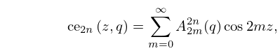
48: 28.4 Fourier Series

… ►

28.4.1 $${\mathrm{ce}}_{2n}(z,q)=\sum _{m=0}^{\mathrm{\infty }}{A}_{2m}^{2n}(q)\cos 2mz,$$

ⓘ

Symbols:

${\mathrm{ce}}_n(z,q)$: Mathieu function, $\cos z$: cosine function, $m$: integer, $q=h^2$: parameter, $n$: integer, $z$: complex variable and $A_m(q)$: Fourier coefficient

A&S Ref:

20.2.3 (in slightly different form) 20.2.4 (in slightly different form)

Permalink:

http://dlmf.nist.gov/28.4.E1

Encodings:

pMML, png, TeX

See also:

Annotations for §28.4(i), §28.4 and Ch.28

… ►

§28.4(iii) Normalization

… ►

§28.4(vi) Behavior for Small $q$

… ►

28.4.21 $$A_{2s}^0(q)=\left(\frac{{(-1)}^{s}2}{{(s!)}^2}{\left(\frac{q}{4}\right)}^s+O\left(q^{s+2}\right)\right)A_0^0(q),$$

ⓘ

Symbols:

$O\left(x\right)$: order not exceeding, $!$: factorial (as in $n!$), $q=h^2$: parameter and $A_m(q)$: Fourier coefficient

A&S Ref:

20.2.29 (in slightly different form)

Permalink:

http://dlmf.nist.gov/28.4.E21

Encodings:

pMML, png, TeX

See also:

Annotations for §28.4(vi), §28.4 and Ch.28

… ►

§28.4(vii) Asymptotic Forms for Large $m$

…

49: Bibliography K

… ►

Closed-form representations of the Lambert $W$ function. Fract. Calc. Appl. Anal. 7 (2), pp. 177–190.

ⓘ

External Links:

ISSN 1311-0454, MathReview (Lewis H. Ryder), ZentralBlatt

Referenced by:

§4.13.

Encodings:

BibTeX

… ►

A vortex filament moving without change of form. J. Fluid Mech. 112, pp. 397–409.

ⓘ

External Links:

ISSN 0022-1120, Document, MathReview, ZentralBlatt

Referenced by:

§19.35(ii).

Encodings:

BibTeX

… ►

Introduction to Elliptic Curves and Modular Forms. 2nd edition, Graduate Texts in Mathematics, Vol. 97, Springer-Verlag, New York.

ⓘ

External Links:

ISBN 0-387-97966-2, MathReview, ZentralBlatt

Referenced by:

§20.10(i), §20.12(i), §20.9(iii), §22.18(iv), §23.1, §23.20(ii), §23.20(v), Ch.23.

Encodings:

BibTeX

… ►

Theta relations and projective normality of Abelian varieties. Amer. J. Math. 98 (4), pp. 865–889.

ⓘ

External Links:

FullText, MathReview (T. Oda), ZentralBlatt

Referenced by:

§21.6(ii).

Encodings:

BibTeX

…

50: 18.35 Pollaczek Polynomials

… ►The Pollaczek polynomials of type 3 are defined by the recurrence relation (in first form (18.2.8)) …or, equivalently in second form (18.2.10), …the recurrence relation of form (18.2.11_5) becomes … ►As in the coefficients of the above recurrence relations $n$ and $c$ only occur in the form $n+c$, the type 3 Pollaczek polynomials may also be called the associated type 2 Pollaczek polynomials by using the terminology of §18.30. … ►

18.35.5 $${\int }_{-1}^1{P}_n^{(\lambda )}(x;a,b)P_m^{(\lambda )}(x;a,b)w^{(\lambda )}(x;a,b)dx=\frac{\mathrm{\Gamma }\left(2\lambda +n\right)}{n!(\lambda +a+n)}{\delta }_{n,m},$$ $a\ge b\ge -a$, $\lambda >0$,

ⓘ

Symbols:

$\mathrm{\Gamma }\left(z\right)$: gamma function, ${\delta }_{j,k}$: Kronecker delta, $P_n^{(\lambda )}(x;a,b)$: Pollaczek polynomial, $dx$: differential of $x$ , $!$: factorial (as in $n!$), $\int$: integral, $w(x)$: weight function, $m$: nonnegative integer, $n$: nonnegative integer and $x$: real variable

Proved:

Ismail (2009, Theorem 5.4.2)(proved)

Referenced by:

(18.35.6), §18.35(ii), Erratum (V1.2.0) for Equation (18.35.5)

Permalink:

http://dlmf.nist.gov/18.35.E5

Encodings:

pMML, png, TeX

Modification (effective with 1.2.0):

This equation which was previously only valid for $n\ne m$, was updated to give the full normalization and the constraints which were originally given in (18.35.6) were moved to this equation. The constraint $\lambda >-\frac{1}{2}$ has been updated to be $\lambda >0$.

See also:

Annotations for §18.35(ii), §18.35 and Ch.18

…