integer%20order

SearchAdvancedHelp

(0.002 seconds)

1—10 of 22 matching pages

1: Bibliography

… ►

Exact linearization of a Painlevé transcendent. Phys. Rev. Lett. 38 (20), pp. 1103–1106.

ⓘ

External Links:

Document, MathReview (Mark Adler)

Referenced by:

§32.11(ii), §32.13(i), §32.13(ii), §32.13(iii), §32.5.

Encodings:

BibTeX

… ►

On the degrees of irreducible factors of higher order Bernoulli polynomials. Acta Arith. 62 (4), pp. 329–342.

ⓘ

External Links:

ISSN 0065-1036, Pdf, MathReview (L. Skula), ZentralBlatt

Referenced by:

§24.12(iii).

Encodings:

BibTeX

►

Congruences of $p$-adic integer order Bernoulli numbers. J. Number Theory 59 (2), pp. 374–388.

ⓘ

External Links:

ISSN 0022-314X, Document, MathReview (L. Skula), ZentralBlatt

Referenced by:

§24.16(iii).

Encodings:

BibTeX

… ►

Algorithm 804: Subroutines for the computation of Mathieu functions of integer orders. ACM Trans. Math. Software 26 (3), pp. 408–414.

ⓘ

Notes:

Double-precision C++, minimum accuracy 14D

External Links:

ISSN 0098-3500, Document, GAMS (module 804; package TOMS)

Referenced by:

1st item, 1st item.

Encodings:

BibTeX

… ►

Spherical Bessel functions $j_n$ and $y_n$ of integer order and real argument. Comput. Phys. Comm. 14 (3-4), pp. 261–265.

ⓘ

Notes:

Single-precision Fortran, maximum accuracy 10S.

External Links:

ISSN 0010-4655, Document, Code

Referenced by:

1st item.

Encodings:

BibTeX

…

2: 26.14 Permutations: Order Notation

§26.14 Permutations: Order Notation

… ►The set ${𝔖}_n$ (§26.13) can be viewed as the collection of all ordered lists of elements of $\{1,2,\mathrm{\dots },n\}$: $\{\sigma (1)\sigma (2)\mathrm{\cdots }\sigma (n)\}$. … ►

26.14.1

ⓘ

Symbols:

$j$: nonnegative integer, $k$: nonnegative integer, $n$: nonnegative integer and $\sigma$: permutation

Permalink:

http://dlmf.nist.gov/26.14.E1

Encodings:

pMML, png, TeX

See also:

Annotations for §26.14(i), §26.14 and Ch.26

►Equivalently, this is the sum over of the number of integers less than $\sigma (j)$ that lie in positions to the right of the $j$th position: $inv(35247816)=2+3+1+1+2+2+0=11.$ … ►

26.14.2

ⓘ

Symbols:

$j$: nonnegative integer, $n$: nonnegative integer, $\sigma$: permutation and $maj(\sigma )$: major index

Permalink:

http://dlmf.nist.gov/26.14.E2

Encodings:

pMML, png, TeX

See also:

Annotations for §26.14(i), §26.14 and Ch.26

…

3: 23.9 Laurent and Other Power Series

… ►

23.9.1 $$c_n=(2n-1)\sum _{w\in 𝕃\setminus \{0\}}{w}^{-2n},$$ $n=2,3,4,\mathrm{\dots }$.

ⓘ

Symbols:

$\in$: element of, $\setminus$: set subtraction, $𝕃$: lattice, $n$: integer and $c_n$

Referenced by:

§20.6

Permalink:

http://dlmf.nist.gov/23.9.E1

Encodings:

pMML, png, TeX

See also:

Annotations for §23.9 and Ch.23

… ►

$c_2={\displaystyle \frac{1}{20}}{g}_2,$

… ►

23.9.5 $$c_n=\frac{3}{(2n+1)(n-3)}\sum _{m=2}^{n-2}{c}_m{c}_{n-m},$$ $n\ge 4$.

ⓘ

Symbols:

$n$: integer, $m$: integer and $c_n$

A&S Ref:

18.5.3

Referenced by:

§23.9

Permalink:

http://dlmf.nist.gov/23.9.E5

Encodings:

pMML, png, TeX

See also:

Annotations for §23.9 and Ch.23

… ►

23.9.6 $$\mathrm{\wp }\left({\omega }_j+t\right)=e_j+(3{e_j}^2-5c_2)t^2+(10c_2{e}_j+21c_3)t^4+(7c_2{e_j}^2+21c_3{e}_j+5c_2^2)t^6+O\left(t^8\right),$$

ⓘ

Symbols:

$O\left(x\right)$: order not exceeding, $\mathrm{\wp }\left(z\right)$ (= $\mathrm{\wp }\left(z|𝕃\right)$ = $\mathrm{\wp }(z;g_2,g_3)$): Weierstrass $\mathrm{\wp }$-function, $e_j$: Weierstrass lattice roots, $𝕃$: lattice, ${\omega }_1$, ${\omega }_3$, ${\omega }_2=-{\omega }_1-{\omega }_3$: lattice generators, $c_n$ and $t$: variable

Referenced by:

§23.9

Permalink:

http://dlmf.nist.gov/23.9.E6

Encodings:

pMML, png, TeX

See also:

Annotations for §23.9 and Ch.23

… ►

23.9.8 $$a_{m,n}=3(m+1)a_{m+1,n-1}+\frac{16}{3}(n+1)a_{m-2,n+1}-\frac{1}{3}(2m+3n-1)(4m+6n-1)a_{m-1,n}.$$

ⓘ

Symbols:

$n$: integer, $m$: integer and $a_{m,n}$: coefficients

A&S Ref:

18.5.8

Permalink:

http://dlmf.nist.gov/23.9.E8

Encodings:

pMML, png, TeX

See also:

Annotations for §23.9 and Ch.23

…

4: Bibliography B

… ►

Algorithms for computing Bessel functions of half-integer order with complex arguments. Zh. Vychisl. Mat. i Mat. Fiz. 28 (10), pp. 1449–1460, 1597.

ⓘ

Notes:

English translation in U.S.S.R. Comput. Math. and Math. Phys. 28(1988), no. 5, 109–117

External Links:

ISSN 0044-4669, Document, MathReview (Walter Gautschi), ZentralBlatt

Referenced by:

§10.77(iv).

Encodings:

BibTeX

… ►

Pionic atoms. Annual Review of Nuclear and Particle Science 20, pp. 467–508.

ⓘ

External Links:

Document

Referenced by:

§33.22(iv).

Encodings:

BibTeX

… ►

Coulomb functions (negative energies). Comput. Phys. Comm. 20 (3), pp. 447–458.

ⓘ

Notes:

Double-precision Fortran code.

External Links:

Document, Code

Referenced by:

1st item, 4th item.

Encodings:

BibTeX

… ►

Bessel Functions. Part II: Functions of Positive Integer Order. British Association for the Advancement of Science, Mathematical Tables, Volume 10, Cambridge University Press, Cambridge.

ⓘ

Notes:

Reprinted, with corrections, in 1960.

External Links:

ISBN 0-521-04321-2, MathReview (R. C. Archibald), ZentralBlatt

Referenced by:

§10.18(iii), §10.19(ii), §10.21(vi), §10.41(ii), 2nd item, 2nd item, §3.6(iii).

Encodings:

BibTeX

… ►

Algorithm 21: Bessel function for a set of integer orders. Comm. ACM 3 (11), pp. 600.

ⓘ

Notes:

Includes Algol code, minimum accuracy 5S. For certification see same journal 8(1965), p. 219.

External Links:

ISSN 0001-0782, Document

Referenced by:

§10.77(ii).

Encodings:

BibTeX

…

5: 26.13 Permutations: Cycle Notation

… ►

26.13.1

ⓘ

Symbols:

$n$: nonnegative integer and $\sigma$: permutation

Permalink:

http://dlmf.nist.gov/26.13.E1

Encodings:

pMML, png, TeX

See also:

Annotations for §26.13 and Ch.26

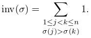
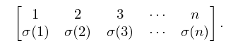
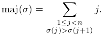
►In cycle notation, the elements in each cycle are put inside parentheses, ordered so that $\sigma (j)$ immediately follows $j$ or, if $j$ is the last listed element of the cycle, then $\sigma (j)$ is the first element of the cycle. … ►An adjacent transposition is a transposition of two consecutive integers. … ►

26.13.5 $$\left(j_1,j_2,\mathrm{\dots },j_k\right)=\left(j_1,j_2\right)\left(j_2,j_3\right)\mathrm{\cdots }\left(j_{k-2},j_{k-1}\right)\left(j_{k-1},j_k\right).$$

ⓘ

Symbols:

$\left(S\right)$: cycle, $j$: nonnegative integer and $k$: nonnegative integer

Permalink:

http://dlmf.nist.gov/26.13.E5

Encodings:

pMML, png, TeX

See also:

Annotations for §26.13 and Ch.26

… ►

26.13.6 $$\left(j,k\right)=\left(k-1,k\right)\left(k-2,k-1\right)\mathrm{\cdots }\left(j+1,j+2\right)\left(j,j+1\right)\left(j+1,j+2\right)\mathrm{\cdots }\left(k-1,k\right).$$

ⓘ

Symbols:

$\left(S\right)$: cycle, $j$: nonnegative integer and $k$: nonnegative integer

Permalink:

http://dlmf.nist.gov/26.13.E6

Encodings:

pMML, png, TeX

See also:

Annotations for §26.13 and Ch.26

…

6: 28.8 Asymptotic Expansions for Large $q$

… ►

28.8.1 $$\begin{array}{c}{a}_m\left(h^2\right)\\ b_{m+1}\left(h^2\right)\end{array}\}\sim -2h^2+2sh-\frac{1}{8}(s^2+1)-\frac{1}{2^{7}h}(s^3+3s)-\frac{1}{2^{12}{h}^2}(5s^4+34s^2+9)-\frac{1}{2^{17}{h}^3}(33s^5+410s^3+405s)-\frac{1}{2^{20}{h}^4}(63s^6+1260s^4+2943s^2+486)-\frac{1}{2^{25}{h}^5}(527s^7+15617s^5+69001s^3+41607s)+\mathrm{\cdots }.$$

ⓘ

Symbols:

$a_n\left(q\right)$: eigenvalues of Mathieu equation, $b_n\left(q\right)$: eigenvalues of Mathieu equation, $\sim$: Poincaré asymptotic expansion, $m$: integer and $h$: parameter

A&S Ref:

20.2.30 (in different form)

Referenced by:

§28.8(i), Erratum (V1.1.10) for Sections 28.6(i), 28.6(ii), 28.8(i), 28.8(ii)

Permalink:

http://dlmf.nist.gov/28.8.E1

Encodings:

pMML, png, TeX

See also:

Annotations for §28.8(i), §28.8 and Ch.28

… ►

28.8.2 $$b_{m+1}\left(h^2\right)-a_m\left(h^2\right)=\frac{2^{4m+5}}{m!}{\left(\frac{2}{\pi }\right)}^{1/2}{h}^{m+(3/2)}{\mathrm{e}}^{-4h}\left(1-\frac{6m^2+14m+7}{32h}+O\left(\frac{1}{h^2}\right)\right).$$

ⓘ

Symbols:

$O\left(x\right)$: order not exceeding, $a_n\left(q\right)$: eigenvalues of Mathieu equation, $b_n\left(q\right)$: eigenvalues of Mathieu equation, $\pi$: the ratio of the circumference of a circle to its diameter, $\mathrm{e}$: base of natural logarithm, $!$: factorial (as in $n!$), $m$: integer and $h$: parameter

A&S Ref:

20.2.31

Permalink:

http://dlmf.nist.gov/28.8.E2

Encodings:

pMML, png, TeX

See also:

Annotations for §28.8(i), §28.8 and Ch.28

… ►

28.8.6 $${\widehat{C}}_m\sim {\left(\frac{\pi h}{2{(m!)}^2}\right)}^{1/4}{\left(1+\frac{2m+1}{8h}+\frac{m^4+2m^3+263m^2+262m+108}{2048h^2}+\mathrm{\cdots }\right)}^{-1/2},$$

ⓘ

Defines:

${\widehat{C}}_m$: coefficient (locally)

Symbols:

$\sim$: Poincaré asymptotic expansion, $\pi$: the ratio of the circumference of a circle to its diameter, $!$: factorial (as in $n!$), $m$: integer and $h$: parameter

A&S Ref:

20.9.19 (in slightly different form)

Permalink:

http://dlmf.nist.gov/28.8.E6

Encodings:

pMML, png, TeX

See also:

Annotations for §28.8(ii), §28.8 and Ch.28

►

28.8.7 $${\widehat{S}}_m\sim {\left(\frac{\pi h}{2{(m!)}^2}\right)}^{1/4}{\left(1-\frac{2m+1}{8h}+\frac{m^4+2m^3-121m^2-122m-84}{2048h^2}+\mathrm{\cdots }\right)}^{-1/2}.$$

ⓘ

Defines:

${\widehat{S}}_m$: coefficient (locally)

Symbols:

$\sim$: Poincaré asymptotic expansion, $\pi$: the ratio of the circumference of a circle to its diameter, $!$: factorial (as in $n!$), $m$: integer and $h$: parameter

A&S Ref:

20.9.20 (in slightly different form)

Referenced by:

§28.8(ii), Erratum (V1.1.10) for Sections 28.6(i), 28.6(ii), 28.8(i), 28.8(ii)

Permalink:

http://dlmf.nist.gov/28.8.E7

Encodings:

pMML, png, TeX

See also:

Annotations for §28.8(ii), §28.8 and Ch.28

… ►

28.8.9 $$W_m^{\pm }(x)=\frac{{\mathrm{e}}^{\pm 2h\sin x}}{{(\cos x)}^{m+1}}\{\begin{array}{cc}{\left(\cos \left(\frac{1}{2}x+\frac{1}{4}\pi \right)\right)}^{2m+1},\hfill & \\ {\left(\sin \left(\frac{1}{2}x+\frac{1}{4}\pi \right)\right)}^{2m+1},\hfill & \end{array}$$

ⓘ

Defines:

$W_m^{\pm }$: function (locally)

Symbols:

$\pi$: the ratio of the circumference of a circle to its diameter, $\cos z$: cosine function, $\mathrm{e}$: base of natural logarithm, $\sin z$: sine function, $m$: integer, $h$: parameter and $x$: real variable

A&S Ref:

20.9.13 (in slightly different form)

Permalink:

http://dlmf.nist.gov/28.8.E9

Encodings:

pMML, png, TeX

See also:

Annotations for §28.8(iii), §28.8 and Ch.28

…

7: 18.40 Methods of Computation

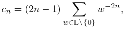
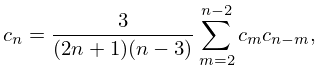
… ►A simple set of choices is spelled out in Gordon (1968) which gives a numerically stable algorithm for direct computation of the recursion coefficients in terms of the moments, followed by construction of the J-matrix and quadrature weights and abscissas, and we will follow this approach: Let $N$ be a positive integer and define … ►

18.40.2 $$a_1={\mu }_0,a_n=\frac{P_{1,n+1}}{P_{1,n}{P}_{1,n-1}},$$ $n=2,\mathrm{\dots },2N+3$,

ⓘ

Symbols:

$N$: positive integer and $n$: nonnegative integer

Permalink:

http://dlmf.nist.gov/18.40.E2

Encodings:

pMML, png, TeX

See also:

Annotations for §18.40(ii), §18.40(ii), §18.40 and Ch.18

… ►

18.40.3 $${\alpha }_0=a_2,{\alpha }_n=a_{2n+1}+a_{2n+2},{\beta }_n=a_{2n}{a}_{2n+1},$$ $n=1,\mathrm{\dots },N$.

ⓘ

Symbols:

$N$: positive integer and $n$: nonnegative integer

Permalink:

http://dlmf.nist.gov/18.40.E3

Encodings:

pMML, png, TeX

See also:

Annotations for §18.40(ii), §18.40(ii), §18.40 and Ch.18

… ►The question is then: how is this possible given only $F_N(z)$, rather than $F(z)$ itself? $F_N(z)$ often converges to smooth results for $z$ off the real axis for $\mathrm{\Im }z$ at a distance greater than the pole spacing of the $x_n$, this may then be followed by approximate numerical analytic continuation via fitting to lower order continued fractions (either Padé, see §3.11(iv), or pointwise continued fraction approximants, see Schlessinger (1968, Appendix)), to $F_N(z)$ and evaluating these on the real axis in regions of higher pole density that those of the approximating function. Results of low ($2$ to $3$ decimal digits) precision for $w(x)$ are easily obtained for $N\sim 10$ to $20$. …

8: 11.6 Asymptotic Expansions

… ►

11.6.1 $${𝐊}_{\nu }\left(z\right)\sim \frac{1}{\pi }\sum _{k=0}^{\mathrm{\infty }}\frac{\mathrm{\Gamma }\left(k+\frac{1}{2}\right){(\frac{1}{2}z)}^{\nu -2k-1}}{\mathrm{\Gamma }\left(\nu +\frac{1}{2}-k\right)},$$ $|\mathrm{ph}z|\le \pi -\delta$,

ⓘ

Symbols:

$\mathrm{\Gamma }\left(z\right)$: gamma function, ${𝐊}_{\nu }\left(z\right)$: Struve function, $\sim$: Poincaré asymptotic expansion, $\pi$: the ratio of the circumference of a circle to its diameter, $\mathrm{ph}$: phase, $z$: complex variable, $\nu$: real or complex order, $k$: nonnegative integer and $\delta$: arbitrary small positive constant

A&S Ref:

12.1.29

Referenced by:

§11.6(i), §11.6(i), §11.6(i), §11.6(i)

Permalink:

http://dlmf.nist.gov/11.6.E1

Encodings:

pMML, png, TeX

See also:

Annotations for §11.6(i), §11.6 and Ch.11

… ►

11.6.2 $${𝐌}_{\nu }\left(z\right)\sim \frac{1}{\pi }\sum _{k=0}^{\mathrm{\infty }}{(-1)}^{k+1}\frac{\mathrm{\Gamma }\left(k+\frac{1}{2}\right){(\frac{1}{2}z)}^{\nu -2k-1}}{\mathrm{\Gamma }\left(\nu +\frac{1}{2}-k\right)},$$ $|\mathrm{ph}z|\le \frac{1}{2}\pi -\delta$.

ⓘ

Symbols:

$\mathrm{\Gamma }\left(z\right)$: gamma function, ${𝐌}_{\nu }\left(z\right)$: modified Struve function, $\sim$: Poincaré asymptotic expansion, $\pi$: the ratio of the circumference of a circle to its diameter, $\mathrm{ph}$: phase, $z$: complex variable, $\nu$: real or complex order, $k$: nonnegative integer and $\delta$: arbitrary small positive constant

A&S Ref:

12.2.6

Referenced by:

§11.6(i), §11.6(i), §11.6(i)

Permalink:

http://dlmf.nist.gov/11.6.E2

Encodings:

pMML, png, TeX

See also:

Annotations for §11.6(i), §11.6 and Ch.11

… ►

§11.6(ii) Large $|\nu |$, Fixed $z$

… ►

11.6.6 $${𝐊}_{\nu }\left(\lambda \nu \right)\sim \frac{{(\frac{1}{2}\lambda \nu )}^{\nu -1}}{\sqrt{\pi }\mathrm{\Gamma }\left(\nu +\frac{1}{2}\right)}\sum _{k=0}^{\mathrm{\infty }}\frac{k!c_k(\lambda )}{{\nu }^k},$$ $|\mathrm{ph}\nu |\le \frac{1}{2}\pi -\delta$,

ⓘ

Symbols:

$\mathrm{\Gamma }\left(z\right)$: gamma function, ${𝐊}_{\nu }\left(z\right)$: Struve function, $\sim$: Poincaré asymptotic expansion, $\pi$: the ratio of the circumference of a circle to its diameter, $!$: factorial (as in $n!$), $\mathrm{ph}$: phase, $\nu$: real or complex order, $k$: nonnegative integer, $\delta$: arbitrary small positive constant, $\lambda$: parameter and $c_k(\lambda )$: expansion function

A&S Ref:

12.1.34

Referenced by:

§11.6(iii)

Permalink:

http://dlmf.nist.gov/11.6.E6

Encodings:

pMML, png, TeX

See also:

Annotations for §11.6(iii), §11.6 and Ch.11

… ►

$c_3(\lambda )=20{\lambda }^{-6}-4{\lambda }^{-4},$

…

9: 6.16 Mathematical Applications

… ►

6.16.2 $$S_n(x)=\sum _{k=0}^{n-1}\frac{\sin \left((2k+1)x\right)}{2k+1}=\frac{1}{2}{\int }_0^x\frac{\sin \left(2nt\right)}{\sin t}dt=\frac{1}{2}\mathrm{Si}\left(2nx\right)+R_n(x),$$

ⓘ

Defines:

$S_n(x)$: partial sum (locally)

Symbols:

$dx$: differential of $x$ , $\int$: integral, $\sin z$: sine function, $\mathrm{Si}\left(z\right)$: sine integral, $x$: real variable, $n$: nonnegative integer and $R_n(x)$: remainder term

Permalink:

http://dlmf.nist.gov/6.16.E2

Encodings:

pMML, png, TeX

See also:

Annotations for §6.16(i), §6.16 and Ch.6

… ►

6.16.3 $$R_n(x)=\frac{1}{2}{\int }_0^x\left(\frac{1}{\sin t}-\frac{1}{t}\right)\sin \left(2nt\right)dt.$$

ⓘ

Defines:

$R_n(x)$: remainder term (locally)

Symbols:

$dx$: differential of $x$ , $\int$: integral, $\sin z$: sine function, $x$: real variable and $n$: nonnegative integer

Permalink:

http://dlmf.nist.gov/6.16.E3

Encodings:

pMML, png, TeX

See also:

Annotations for §6.16(i), §6.16 and Ch.6

… ►

6.16.4 $$R_n(x)=O\left(n^{-1}\right),$$ $n\to \mathrm{\infty }$,

ⓘ

Symbols:

$O\left(x\right)$: order not exceeding, $x$: real variable, $n$: nonnegative integer and $R_n(x)$: remainder term

Permalink:

http://dlmf.nist.gov/6.16.E4

Encodings:

pMML, png, TeX

See also:

Annotations for §6.16(i), §6.16 and Ch.6

… ►

6.16.5 $$\mathrm{li}\left(x\right)-\pi (x)=O\left(\sqrt{x}\ln x\right),$$ $x\to \mathrm{\infty }$,

ⓘ

Symbols:

$O\left(x\right)$: order not exceeding, $\mathrm{li}\left(x\right)$: logarithmic integral, $\ln z$: principal branch of logarithm function, $x$: real variable and $\pi (x)$: number of primes $\le x$

A&S Ref:

5.1.50

Permalink:

http://dlmf.nist.gov/6.16.E5

Encodings:

pMML, png, TeX

See also:

Annotations for §6.16(ii), §6.16 and Ch.6

… ►

►►

Figure 6.16.2: The logarithmic integral $\mathrm{li}\left(x\right)$, together with vertical bars indicating the value of $\pi (x)$ for $x=10,20,\mathrm{\dots },1000$. Magnify

10: 18.39 Applications in the Physical Sciences

… ►The nature of, and notations and common vocabulary for, the eigenvalues and eigenfunctions of self-adjoint second order differential operators is overviewed in §1.18. … ►The fundamental quantum Schrödinger operator, also called the Hamiltonian, $\mathscr{H}$, is a second order differential operator of the form … ► ${ϵ}_0$ is referred to as the ground state, all others, $n=1,2,\mathrm{\dots },$ in order of increasing energy being excited states. … ►Namely the $k$th eigenfunction, listed in order of increasing eigenvalues, starting at $k=0$, has precisely $k$ nodes, as real zeros of wave-functions away from boundaries are often referred to. … ►Derivations of (18.39.42) appear in Bethe and Salpeter (1957, pp. 12–20), and Pauling and Wilson (1985, Chapter V and Appendix VII), where the derivations are based on (18.39.36), and is also the notation of Piela (2014, §4.7), typifying the common use of the associated Coulomb–Laguerre polynomials in theoretical quantum chemistry. …