infinite%20partial%20fractions

SearchAdvancedHelp

(0.002 seconds)

11—20 of 311 matching pages

11: 18.39 Applications in the Physical Sciences

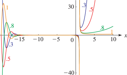
… ►with an infinite set of orthonormal $L^2$ eigenfunctions … ►This indicates that the Laguerre polynomials appearing in (18.39.29) are not classical OP’s, and in fact, even though infinite in number for fixed $l$, do not form a complete set. Namely for fixed $l$ the infinite set labeled by $p$ describe only the $L^2$ bound states for that single $l$, omitting the continuum briefly mentioned below, and which is the subject of Chapter 33, and so an unusual example of the mixed spectra of §1.18(viii). … ►Derivations of (18.39.42) appear in Bethe and Salpeter (1957, pp. 12–20), and Pauling and Wilson (1985, Chapter V and Appendix VII), where the derivations are based on (18.39.36), and is also the notation of Piela (2014, §4.7), typifying the common use of the associated Coulomb–Laguerre polynomials in theoretical quantum chemistry. … ►These, taken together with the infinite sets of bound states for each $l$, form complete sets. …

12: Bibliography S

… ►

Transformations of the Jacobian amplitude function and its calculation via the arithmetic-geometric mean. SIAM J. Math. Anal. 20 (6), pp. 1514–1528.

ⓘ

External Links:

ISSN 0036-1410, Document, MathReview (J. M. H. Peters), ZentralBlatt

Referenced by:

§22.19(i), §22.20(vi).

Encodings:

BibTeX

… ►

On integral representation of Weber’s parabolic cylinder function and its expansion into an infinite series. J. Indian Math. Soc. (N. S.) 4, pp. 34–38.

ⓘ

External Links:

MathReview (M. C. Gray), ZentralBlatt

Referenced by:

§12.13(ii).

Encodings:

BibTeX

… ►

Uniform asymptotic forms of modified Mathieu functions. Quart. J. Mech. Appl. Math. 20 (3), pp. 365–380.

ⓘ

External Links:

Document, MathReview (F. W. J. Olver), ZentralBlatt

Referenced by:

§28.8(iv).

Encodings:

BibTeX

… ►

Computation of infinite integrals involving Bessel functions of arbitrary order by the $\overline{D}$-transformation. J. Comput. Appl. Math. 78 (1), pp. 125–130.

ⓘ

External Links:

ISSN 0377-0427, Document, MathReview, ZentralBlatt

Referenced by:

§10.74(vii).

Encodings:

BibTeX

… ►

A Maple package for symmetric functions. J. Symbolic Comput. 20 (5-6), pp. 755–768.

ⓘ

Notes:

For software see John Stembridge’s home page. The SF package contains Maple software for zonal, Jack, and Macdonald polynomials.

External Links:

Home Page, ISSN 0747-7171, Document, MathReview, ZentralBlatt

Referenced by:

3rd item.

Encodings:

BibTeX

…

13: 3.4 Differentiation

… ►

§3.4(iii) Partial Derivatives

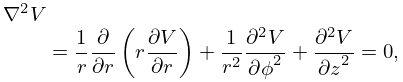
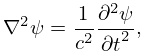
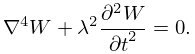
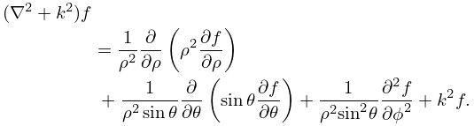
… ► … ►The results in this subsection for the partial derivatives follow from Panow (1955, Table 10). Those for the Laplacian and the biharmonic operator follow from the formulas for the partial derivatives. … ►

14: 36.4 Bifurcation Sets

… ►

36.4.1 $$\frac{\partial }{\partial t}{\mathrm{\Phi }}_K(t_j(𝐱);𝐱)=0.$$

ⓘ

Symbols:

${\mathrm{\Phi }}_K(t;𝐱)$: cuspoid catastrophe of codimension $K$ , $\frac{\partial f}{\partial x}$: partial derivative of $f$ with respect to $x$ , $\partial x$: partial differential of $x$ , $t$: variable, $K$: codimension and $t_j(𝐱)$: solutions

Referenced by:

§36.11, §36.12(i), §36.4(i), §36.5(i), §36.5(ii)

Permalink:

http://dlmf.nist.gov/36.4.E1

Encodings:

pMML, png, TeX

See also:

Annotations for §36.4(i), §36.4(i), §36.4 and Ch.36

… ►

36.4.3 $$\frac{{\partial }^2}{{\partial t}^2}{\mathrm{\Phi }}_K(t;𝐱)=0.$$

ⓘ

Symbols:

${\mathrm{\Phi }}_K(t;𝐱)$: cuspoid catastrophe of codimension $K$ , $\frac{\partial f}{\partial x}$: partial derivative of $f$ with respect to $x$ , $\partial x$: partial differential of $x$ , $t$: variable and $K$: codimension

Permalink:

http://dlmf.nist.gov/36.4.E3

Encodings:

pMML, png, TeX

See also:

Annotations for §36.4(i), §36.4(i), §36.4 and Ch.36

… ►

36.4.4

ⓘ

Symbols:

$\frac{\partial f}{\partial x}$: partial derivative of $f$ with respect to $x$ , $\partial x$: partial differential of $x$ , : elliptic umbilic catastrophe for $\mathrm{U}=\mathrm{E}\text{ or }\mathrm{K}$ , $t$: variable and $s$: variable

Permalink:

http://dlmf.nist.gov/36.4.E4

Encodings:

pMML, png, TeX

See also:

Annotations for §36.4(i), §36.4(i), §36.4 and Ch.36

… ►

$x=\frac{9}{20}{z}^2.$

… ►

$x=-\frac{3}{20}{z}^2,$

…

15: 27.2 Functions

… ►Euclid’s Elements (Euclid (1908, Book IX, Proposition 20)) gives an elegant proof that there are infinitely many primes. … ►

Table 27.2.2: Functions related to division.

► ►►►►►►

$n$	$\varphi \left(n\right)$	$d\left(n\right)$	$\sigma \left(n\right)$	$n$	$\varphi \left(n\right)$	$d\left(n\right)$	$\sigma \left(n\right)$	$n$	$\varphi \left(n\right)$	$d\left(n\right)$	$\sigma \left(n\right)$	$n$	$\varphi \left(n\right)$	$d\left(n\right)$	$\sigma \left(n\right)$
…
5	4	2	6	18	6	6	39	31	30	2	32	44	20	6	84
6	2	4	12	19	18	2	20	32	16	6	63	45	24	6	78
7	6	2	8	20	8	6	42	33	20	4	48	46	22	4	72
…
11	10	2	12	24	8	8	60	37	36	2	38	50	20	6	93
…

►

16: 25.11 Hurwitz Zeta Function

… ►

►►

Figure 25.11.1: Hurwitz zeta function $\zeta (x,a)$, $a$ = 0. …8, 1, $-20\le x\le 10$. … Magnify

… ►

25.11.8 $$\zeta (s,\frac{1}{2}a)=\zeta (s,\frac{1}{2}a+\frac{1}{2})+2^s\sum _{n=0}^{\mathrm{\infty }}\frac{{(-1)}^n}{{(n+a)}^s},$$ $\mathrm{\Re }s>0$, $s\ne 1$, .

ⓘ

Symbols:

$\zeta (s,a)$: Hurwitz zeta function, $\mathrm{\Re }$: real part, $n$: nonnegative integer, $a$: real or complex parameter and $s$: complex variable

Keywords:

infinite series, series representation

Source:

Srivastava and Choi (2001, (5), p. 89)

Referenced by:

(25.11.35), §25.11(x)

Permalink:

http://dlmf.nist.gov/25.11.E8

Encodings:

pMML, png, TeX

See also:

Annotations for §25.11(iv), §25.11 and Ch.25

… ►

25.11.35 $$\sum _{n=0}^{\mathrm{\infty }}\frac{{(-1)}^n}{{(n+a)}^s}=\frac{1}{\mathrm{\Gamma }\left(s\right)}{\int }_0^{\mathrm{\infty }}\frac{x^{s-1}{\mathrm{e}}^{-ax}}{1+{\mathrm{e}}^{-x}}dx=2^{-s}\left(\zeta (s,\frac{1}{2}a)-\zeta (s,\frac{1}{2}(1+a))\right),$$ $\mathrm{\Re }a>0$, $\mathrm{\Re }s>0$; or $\mathrm{\Re }a=0$, $\mathrm{\Im }a\ne 0$, .

ⓘ

Symbols:

$\mathrm{\Gamma }\left(z\right)$: gamma function, $\zeta (s,a)$: Hurwitz zeta function, $dx$: differential of $x$ , $\mathrm{e}$: base of natural logarithm, $\mathrm{\Im }$: imaginary part, $\int$: integral, $\mathrm{\Re }$: real part, $n$: nonnegative integer, $x$: real variable, $a$: real or complex parameter and $s$: complex variable

Keywords:

improper integral, infinite series, integral representation, series representation

Proof sketch:

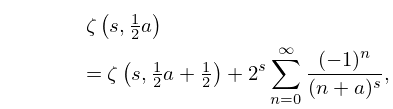
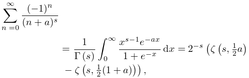
The infinite series connection to the difference of Hurwitz zeta functions is a restatement of (25.11.8). The integral representation is derivable from the difference of Hurwitz zeta functions by substituting (25.11.25) in each, making a change of variables $x=2t$, factoring, and expressing $1-{\mathrm{e}}^{-2t}=(1+{\mathrm{e}}^{-t})(1-{\mathrm{e}}^{-t})$.

Referenced by:

(25.11.31), §25.11(x), §25.11(x)

Permalink:

http://dlmf.nist.gov/25.11.E35

Encodings:

pMML, png, TeX

See also:

Annotations for §25.11(x), §25.11 and Ch.25

… ►

25.11.38 $$\sum _{k=1}^{\mathrm{\infty }}\left(\genfrac{}{}{0.0pt}{}{n+k}{k}\right)\zeta (n+k+1,a)z^k=\frac{{(-1)}^n}{n!}\left({\psi }^{(n)}\left(a\right)-{\psi }^{(n)}\left(a-z\right)\right),$$ $n=1,2,3,\mathrm{\dots }$, $\mathrm{\Re }a>0$, .

ⓘ

Symbols:

$\zeta (s,a)$: Hurwitz zeta function, $\left(\genfrac{}{}{0.0pt}{}{m}{n}\right)$: binomial coefficient, $\psi \left(z\right)$: psi (or digamma) function, $!$: factorial (as in $n!$), $\mathrm{\Re }$: real part, $k$: nonnegative integer, $n$: nonnegative integer, $a$: real or complex parameter and $z$: complex variable

Keywords:

infinite series, series representation

Source:

Adamchik and Srivastava (1998, (2.29), p. 138)

Permalink:

http://dlmf.nist.gov/25.11.E38

Encodings:

pMML, png, TeX

See also:

Annotations for §25.11(xi), §25.11 and Ch.25

►

25.11.39 $$\sum _{k=2}^{\mathrm{\infty }}\frac{k}{2^k}\zeta (k+1,\frac{3}{4})=8G,$$

ⓘ

Symbols:

$\zeta (s,a)$: Hurwitz zeta function, $k$: nonnegative integer and $G$: Catalan’s constant

Keywords:

Catalan’s constant, infinite series

Source:

Adamchik and Srivastava (1998, (2.30), p. 138)

Permalink:

http://dlmf.nist.gov/25.11.E39

Encodings:

pMML, png, TeX

See also:

Annotations for §25.11(xi), §25.11 and Ch.25

…

17: 10.73 Physical Applications

… ►

10.73.1 $${\nabla }^{2}V=\frac{1}{r}\frac{\partial }{\partial r}\left(r\frac{\partial V}{\partial r}\right)+\frac{1}{r^2}\frac{{\partial }^{2}V}{{\partial \varphi }^2}+\frac{{\partial }^{2}V}{{\partial z}^2}=0,$$

ⓘ

Symbols:

$\frac{\partial f}{\partial x}$: partial derivative of $f$ with respect to $x$ and $\partial x$: partial differential of $x$

Permalink:

http://dlmf.nist.gov/10.73.E1

Encodings:

pMML, png, TeX

See also:

Annotations for §10.73(i), §10.73 and Ch.10

… ►

10.73.2 $${\nabla }^2\psi =\frac{1}{c^2}\frac{{\partial }^2\psi }{{\partial t}^2},$$

ⓘ

Symbols:

$\frac{\partial f}{\partial x}$: partial derivative of $f$ with respect to $x$ and $\partial x$: partial differential of $x$

Permalink:

http://dlmf.nist.gov/10.73.E2

Encodings:

pMML, png, TeX

See also:

Annotations for §10.73(i), §10.73 and Ch.10

… ►See Krivoshlykov (1994, Chapter 2, §2.2.10; Chapter 5, §5.2.2), Kapany and Burke (1972, Chapters 4–6; Chapter 7, §A.1), and Slater (1942, Chapter 4, §§20, 25). … ►

10.73.3 $${\nabla }^{4}W+{\lambda }^2\frac{{\partial }^{2}W}{{\partial t}^2}=0.$$

ⓘ

Symbols:

$\frac{\partial f}{\partial x}$: partial derivative of $f$ with respect to $x$ and $\partial x$: partial differential of $x$

Permalink:

http://dlmf.nist.gov/10.73.E3

Encodings:

pMML, png, TeX

See also:

Annotations for §10.73(i), §10.73 and Ch.10

… ►

10.73.4 $$({\nabla }^2+k^2)f=\frac{1}{{\rho }^2}\frac{\partial }{\partial \rho }\left({\rho }^2\frac{\partial f}{\partial \rho }\right)+\frac{1}{{\rho }^2\sin \theta }\frac{\partial }{\partial \theta }\left(\sin \theta \frac{\partial f}{\partial \theta }\right)+\frac{1}{{\rho }^2{\sin }^2\theta }\frac{{\partial }^{2}f}{{\partial \varphi }^2}+k^{2}f.$$

ⓘ

Symbols:

$\frac{\partial f}{\partial x}$: partial derivative of $f$ with respect to $x$ , $\partial x$: partial differential of $x$ , $\sin z$: sine function and $k$: nonnegative integer

Permalink:

http://dlmf.nist.gov/10.73.E4

Encodings:

pMML, png, TeX

See also:

Annotations for §10.73(ii), §10.73 and Ch.10

…

18: Bibliography L

… ►

An asymptotic estimate for the Bernoulli and Euler numbers. Canad. Math. Bull. 20 (1), pp. 109–111.

ⓘ

External Links:

MathReview (D. H. Lehmer), ZentralBlatt

Referenced by:

§24.11.

Encodings:

BibTeX

… ►

On the theory of diffraction by an aperture in an infinite plane screen. I. Phys. Rev. 74 (8), pp. 958–974.

ⓘ

External Links:

Document, MathReview (C. J. Bouwkamp), ZentralBlatt

Referenced by:

§11.12.

Encodings:

BibTeX

… ►

Note on a method for computing infinite integrals of oscillatory functions. Proc. Cambridge Philos. Soc. 52 (4), pp. 764–768.

ⓘ

External Links:

Document, MathReview (D. J. Hofsommer), ZentralBlatt

Referenced by:

§3.5(vii).

Encodings:

BibTeX

… ►

Evaluating infinite integrals involving Bessel functions of arbitrary order. J. Comput. Appl. Math. 64 (3), pp. 217–231.

ⓘ

External Links:

ISSN 0377-0427, Document, MathReview Entry, ZentralBlatt

Referenced by:

§10.74(vii).

Encodings:

BibTeX

… ►

Integrating some infinite oscillating tails. J. Comput. Appl. Math. 12/13, pp. 109–117.

ⓘ

External Links:

ISSN 0377-0427, Document, MathReview Entry, ZentralBlatt

Referenced by:

§3.5(vii).

Encodings:

BibTeX

19: 5.19 Mathematical Applications

… ►As shown in Temme (1996b, §3.4), the results given in §5.7(ii) can be used to sum infinite series of rational functions. … ►By decomposition into partial fractions (§1.2(iii)) … ►Many special functions $f(z)$ can be represented as a Mellin–Barnes integral, that is, an integral of a product of gamma functions, reciprocals of gamma functions, and a power of $z$, the integration contour being doubly-infinite and eventually parallel to the imaginary axis at both ends. …

20: 22.12 Expansions in Other Trigonometric Series and Doubly-Infinite Partial Fractions: Eisenstein Series

§22.12 Expansions in Other Trigonometric Series and Doubly-Infinite Partial Fractions: Eisenstein Series

… ►

22.12.13 $$2K\mathrm{cs}(2Kt,k)=\underset{N\to \mathrm{\infty }}{lim}\sum _{n=-N}^N{(-1)}^n\frac{\pi }{\tan \left(\pi (t-n\tau )\right)}=\underset{N\to \mathrm{\infty }}{lim}\sum _{n=-N}^N{(-1)}^n\left(\underset{M\to \mathrm{\infty }}{lim}\sum _{m=-M}^M\frac{1}{t-m-n\tau }\right).$$

ⓘ

Symbols:

$\mathrm{cs}(z,k)$: Jacobian elliptic function, $\pi$: the ratio of the circumference of a circle to its diameter, $K\left(k\right)$: Legendre’s complete elliptic integral of the first kind, $\tan z$: tangent function, $k$: modulus and $\tau$: ratio

Referenced by:

§22.12

Permalink:

http://dlmf.nist.gov/22.12.E13

Encodings:

pMML, png, TeX

See also:

Annotations for §22.12 and Ch.22