graphs of solutions

SearchAdvancedHelp

(0.002 seconds)

11—20 of 22 matching pages

11: 2.11 Remainder Terms; Stokes Phenomenon

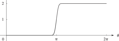
… ►In the transition through $\theta =\pi$, $\mathrm{erfc}\left(\sqrt{\frac{1}{2}\rho }c(\theta )\right)$ changes very rapidly, but smoothly, from one form to the other; compare the graph of its modulus in Figure 2.11.1 in the case $\rho =100$. ►

►►

Figure 2.11.1: Graph of $|\mathrm{erfc}\left(\sqrt{50}c(\theta )\right)|$. Magnify

… ►As these lines are crossed exponentially-small contributions, such as that in (2.11.7), are “switched on” smoothly, in the manner of the graph in Figure 2.11.1. … ►

§2.11(v) Exponentially-Improved Expansions (continued)

… ►

2.11.19 $$w_j(z)={\mathrm{e}}^{{\lambda }_{j}z}{z}^{{\mu }_j}\sum _{s=0}^{n-1}\frac{a_{s,j}}{z^s}+R_n^{(j)}(z),$$ $j=1,2$,

ⓘ

Symbols:

$\mathrm{e}$: base of natural logarithm, $R_n^{(j)}(z)$: remainder, $a_{s,j}$: coefficients, ${\lambda }_j$: roots, ${\mu }_j$: quantities and $w_j(z)$: solutions

Permalink:

http://dlmf.nist.gov/2.11.E19

Encodings:

pMML, png, TeX

See also:

Annotations for §2.11(v), §2.11 and Ch.2

…

12: 10.45 Functions of Imaginary Order

… ►and ${\tilde{I}}_{\nu }\left(x\right)$, ${\tilde{K}}_{\nu }\left(x\right)$ are real and linearly independent solutions of (10.45.1): … ►In consequence of (10.45.5)–(10.45.7), ${\tilde{I}}_{\nu }\left(x\right)$ and ${\tilde{K}}_{\nu }\left(x\right)$ comprise a numerically satisfactory pair of solutions of (10.45.1) when $x$ is large, and either ${\tilde{I}}_{\nu }\left(x\right)$ and $(1/\pi )\sinh \left(\pi \nu \right){\tilde{K}}_{\nu }\left(x\right)$, or ${\tilde{I}}_{\nu }\left(x\right)$ and ${\tilde{K}}_{\nu }\left(x\right)$, comprise a numerically satisfactory pair when $x$ is small, depending whether $\nu \ne 0$ or $\nu =0$. … ►For graphs of ${\tilde{I}}_{\nu }\left(x\right)$ and ${\tilde{K}}_{\nu }\left(x\right)$ see §10.26(iii). …

13: 10.24 Functions of Imaginary Order

… ►and ${\tilde{J}}_{\nu }\left(x\right)$, ${\tilde{Y}}_{\nu }\left(x\right)$ are linearly independent solutions of (10.24.1): … ►In consequence of (10.24.6), when $x$ is large ${\tilde{J}}_{\nu }\left(x\right)$ and ${\tilde{Y}}_{\nu }\left(x\right)$ comprise a numerically satisfactory pair of solutions of (10.24.1); compare §2.7(iv). … ►For graphs of ${\tilde{J}}_{\nu }\left(x\right)$ and ${\tilde{Y}}_{\nu }\left(x\right)$ see §10.3(iii). …

14: 9.12 Scorer Functions

… ►The general solution is given by …Standard particular solutions are … ►

§9.12(ii) Graphs

… ►

§9.12(iv) Numerically Satisfactory Solutions

… ►In $ℂ$, numerically satisfactory sets of solutions are given by …

15: 12.14 The Function $W(a,x)$

… ►

§12.14(i) Introduction

►In this section solutions of equation (12.2.3) are considered. … ►

§12.14(iii) Graphs

… ►The even and odd solutions of (12.2.3) (see §12.14(v)) are given by … ►For graphs of the modulus functions see §12.14(iii). …

16: 14.20 Conical (or Mehler) Functions

… ►Solutions are known as conical or Mehler functions. … ►Another real-valued solution ${\widehat{𝖰}}_{-\frac{1}{2}+\mathrm{i}\tau }^{-\mu }\left(x\right)$ of (14.20.1) was introduced in Dunster (1991). …It is an important companion solution to ${𝖯}_{-\frac{1}{2}+\mathrm{i}\tau }^{-\mu }\left(x\right)$ when $\tau$ is large; compare §§14.20(vii), 14.20(viii), and 10.25(iii). … ►Lastly, for the range , $P_{-\frac{1}{2}+\mathrm{i}\tau }^{-\mu }\left(x\right)$ is a real-valued solution of (14.20.1); in terms of $Q_{-\frac{1}{2}\pm \mathrm{i}\tau }^{\mu }\left(x\right)$ (which are complex-valued in general): …

17: Bibliography

… ►

Asymptotics of solutions of the generalized sine-Gordon equation, the third Painlevé equation and the d’Alembert equation. Dokl. Akad. Nauk SSSR 280 (2), pp. 265–268 (Russian).

ⓘ

Notes:

English translation: Soviet Math. Dokl. 31(1985), no. 1, pp. 45–47

External Links:

ISSN 0002-3264, MathReview (M. S. Agranovich), ZentralBlatt

Referenced by:

§32.11(iv).

Encodings:

BibTeX

… ►

Handbook of Mathematical Functions with Formulas, Graphs, and Mathematical Tables. National Bureau of Standards Applied Mathematics Series, U.S. Government Printing Office, Washington, D.C..

ⓘ

Notes:

Corrections appeared in later printings up to the 10th Printing, December, 1972. Reproductions by other publishers, in whole or in part, have been available since 1965.

External Links:

FullText, MathReview (D. H. Lehmer), ZentralBlatt

Referenced by:

§10.1, §10.21(ix), §10.47(i), §10.68(iv), §10.70, 4th item, 2nd item, 4th item, 5th item, 1st item, 1st item, 4th item, 1st item, 1st item, Ch.10, §11.10(vi), 1st item, 1st item, Ch.11, 1st item, Ch.12, 3rd item, Ch.13, 1st item, Ch.14, Ch.15, §18.14(i), §18.3, §18.41(i), §18.41(ii), §18.5(iv), §18.8, §19.1, §19.14(i), §19.14(ii), §19.25(v), §19.36(iii), §19.37(ii), §19.37(ii), §19.37(ii), §19.37(ii), §19.37(iii), §19.37(iii), §19.38, Ch.19, §20.15, Ch.20, §22.1, §22.15(ii), Ch.22, §23.1, §23.20(i), §23.23, §23.23, §23.9, §23.9, §23.9, Ch.23, §24.2(iv), §24.20, Ch.24, 1st item, §26.1, §26.1, §26.2, §26.21, §26.3(i), §26.4(i), §26.8(i), §27.2(ii), §27.21, §28.1, Ch.28, §30.1, Ch.30, 1st item, Ch.33, §4.44, §4.46, §5.11(i), §5.22(ii), §5.22(iii), §5.7(i), Ch.5, 1st item, 1st item, 1st item, Ch.6, 1st item, 2nd item, 1st item, Ch.7, (8.17.24), §8.22(ii), 1st item, Ch.8, 1st item, 1st item, 1st item, §9.8(i), Ch.9, Profile Frank W. J. Olver, About the Project, Preface, Possible Errors in DLMF, Notations E, Notations E, Notations F, Notations F, Notations H, Notations H, Notations J, Notations K, Notations P, Notations P, Notations S, Notations Y, H. E. Fettis and J. C. Caslin (1973).

Encodings:

BibTeX

… ►

Rational solutions of Painlevé equations. Stud. Appl. Math. 61 (1), pp. 31–53.

ⓘ

External Links:

ISSN 0022-2526, MathReview (H. Hochstadt), ZentralBlatt

Referenced by:

§32.10(ii), §32.8(i), §32.8(v).

Encodings:

BibTeX

… ►

Perturbation solutions of the ellipsoidal wave equation. Quart. J. Math. Oxford Ser. (2) 7, pp. 161–174.

ⓘ

External Links:

ISSN 0033-5606, Document, MathReview (A. Erdélyi), ZentralBlatt

Referenced by:

§29.11.

Encodings:

BibTeX

… ►

Graphs as an Aid to Understanding Special Functions. In Asymptotic and Computational Analysis, R. Wong (Ed.), Lecture Notes in Pure and Appl. Math., Vol. 124, pp. 3–33.

ⓘ

External Links:

MathReview Entry, ZentralBlatt

Referenced by:

§18.14(iii), Figure 18.4.2, Figure 18.4.2.

Encodings:

BibTeX

…

18: 3.8 Nonlinear Equations

§3.8 Nonlinear Equations

… ►Solutions are called roots of the equation, or zeros of $f$. … ►and the solutions are called fixed points of $\varphi$. … ►From this graph we estimate an initial value $x_0=4.65$. … ►For describing the distribution of complex zeros of solutions of linear homogeneous second-order differential equations by methods based on the Liouville–Green (WKB) approximation, see Segura (2013). …

19: 12.2 Differential Equations

§12.2 Differential Equations

… ►PCFs are solutions of the differential equation … ►All solutions are entire functions of $z$ and entire functions of $a$ or $\nu$. … ►The solutions $W(a,\pm x)$ are treated in §12.14. … ►For graphs of the modulus functions see §12.3(i).

20: 18.39 Applications in the Physical Sciences

… ►The solutions of (18.39.8) are subject to boundary conditions at $a$ and $b$. … ►The solutions (18.39.8) are called the stationary states as separation of variables in (18.39.9) yields solutions of form … ►Brief mention of non-unit normalized solutions in the case of mixed spectra appear, but as these solutions are not OP’s details appear elsewhere, as referenced. … ►The radial Coulomb wave functions $R_{n,l}(r)$, solutions of … ►Graphs of the weight functions of (18.39.50) are shown in Figure 18.39.2. …