generalized hypergeometric differential equation
(0.005 seconds)
41—50 of 55 matching pages
41: 15.2 Definitions and Analytical Properties
…
►
§15.2(i) Gauss Series
… ►In general, does not exist when . … ►§15.2(ii) Analytic Properties
… ►The same properties hold for , except that as a function of , in general has poles at . … ►(Both interpretations give solutions of the hypergeometric differential equation (15.10.1), as does , which is analytic at .) …42: 19.20 Special Cases
…
►
19.20.2
…
►The general lemniscatic case is
…
►
19.20.22
…
►The general
lemniscatic case is
…
►
19.20.25
…
43: Bibliography R
…
►
Uniform asymptotic approximations to the solutions of the Orr-Sommerfeld equation. II. The general theory.
Studies in Appl. Math. 53, pp. 217–224.
…
►
Total positivity properties of generalized hypergeometric functions of matrix argument.
J. Statist. Phys. 116 (1-4), pp. 907–922.
…
►
Research Institute for Symbolic Computation, Hagenberg im Mühlkreis, Austria.
…
►
Heun’s Differential Equations.
The Clarendon Press Oxford University Press, New York.
…
►
Elliptic hypergeometric series on root systems.
Adv. Math. 181 (2), pp. 417–447.
…
44: Bibliography Z
…
►
On the Computation of Zeros of Bessel and Bessel-related Functions.
In Proceedings of the Sixth International Colloquium on
Differential Equations (Plovdiv, Bulgaria, 1995), D. Bainov (Ed.),
Utrecht, pp. 409–416.
…
►
Distribution of zeros of Gauss and Kummer hypergeometric functions. A semiclassical approach.
Ann. Numer. Math. 2 (1-4), pp. 457–472.
…
►
Doron Zeilberger’s Maple Packages and Programs
Department of Mathematics, Rutgers University, New Jersey.
►
Distribution Theory and Transform Analysis, An Introduction and Generalized Functions with Applications.
Dover, New York.
…
►
Generalized Watson Transforms and Applications to Group Representations.
Ph.D. Thesis, University of Vermont, Burlington,VT.
…
45: 13.2 Definitions and Basic Properties
…
►
§13.2(i) Differential Equation
►Kummer’s Equation
… ►It can be regarded as the limiting form of the hypergeometric differential equation (§15.10(i)) that is obtained on replacing by , letting , and subsequently replacing the symbol by . In effect, the regular singularities of the hypergeometric differential equation at and coalesce into an irregular singularity at . … ►In general, has a branch point at . …46: Bibliography F
…
►
Computation of complex Airy functions and their zeros using asymptotics and the differential equation.
ACM Trans. Math. Software 30 (4), pp. 471–490.
…
►
Generalized parabolic cylinder functions.
Asymptotic Anal. 5 (6), pp. 517–531.
►
Theory and Computation of Spheroidal Harmonics with General Arguments.
Master’s Thesis, The University of Western Australia, Department of Physics.
…
►
Expansions of hypergeometric functions in hypergeometric functions.
Math. Comp. 15 (76), pp. 390–395.
…
►
Finite Differences and Difference Equations in the Real Domain.
Clarendon Press, Oxford.
…
47: 33.14 Definitions and Basic Properties
…
►
§33.14(i) Coulomb Wave Equation
… ►§33.14(ii) Regular Solution
… ►where and are defined in §§13.14(i) and 13.2(i), and … ►For nonzero values of and the function is defined by … ►
33.14.15
…
48: Mathematical Introduction
…
►These include, for example, multivalued functions of complex variables, for which new definitions of branch points and principal values are supplied (§§1.10(vi), 4.2(i)); the Dirac delta (or delta function), which is introduced in a more readily comprehensible way for mathematicians (§1.17); numerically satisfactory solutions of differential and difference equations (§§2.7(iv), 2.9(i)); and numerical analysis for complex variables (Chapter 3).
…
►For example, for the hypergeometric function we often use the notation (§15.2(i)) in place of the more conventional or .
This is because is akin to the notation used for Bessel functions (§10.2(ii)), inasmuch as is an entire function of each of its parameters , , and : this results in fewer restrictions and simpler equations.
Similarly in the case of confluent hypergeometric functions (§13.2(i)).
…
►For equations or other technical information that appeared previously in AMS 55, the DLMF usually includes the corresponding AMS 55 equation number, or other form of reference, together with corrections, if needed.
…
49: 13.16 Integral Representations
…
►In this subsection see §§10.2(ii), 10.25(ii) for the functions , , and , and §§15.1, 15.2(i) for .
…
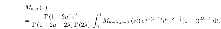
►
13.16.2
,
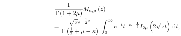
►
13.16.3
,
►
13.16.4
.
…
►
13.16.9
,
…
50: 13.14 Definitions and Basic Properties
…
►
