cosine%20integrals
(0.002 seconds)
11—16 of 16 matching pages
11: Software Index
…
►
►
…
| Open Source | With Book | Commercial | |||||||||||||||||||||||
| … | |||||||||||||||||||||||||
| 6 Exponential, Logarithmic, Sine, and Cosine Integrals | |||||||||||||||||||||||||
| 6.21(ii) , , , , , , | ✓ | ✓ | ✓ | ✓ | ✓ | ✓ | ✓ | ✓ | ✓ | ✓ | ✓ | ✓ | ✓ | ✓ | ✓ | ✓ | ✓ | ✓ | ✓ | ✓ | ✓ | ✓ | |||
| 6.21(iii) , , , , , | ✓ | ✓ | ✓ | ✓ | ✓ | ✓ | ✓ | ✓ | ✓ | ✓ | |||||||||||||||
| … | |||||||||||||||||||||||||
| 7.25(v) , , | ✓ | a | ✓ | ✓ | ✓ | ✓ | |||||||||||||||||||
| … | |||||||||||||||||||||||||
| 20 Theta Functions | |||||||||||||||||||||||||
| … | |||||||||||||||||||||||||
12: Errata
…
►
Equation (18.28.8)
…
►
Subsection 19.11(i)
…
►
Section 1.14
…
►
Chapters 8, 20, 36
…
►
References
…
18.28.8
or ; ;
The constraint which originally stated that “” has been updated to be “”.
A sentence and unnumbered equation
were added which indicate that care must be taken with the multivalued functions in (19.11.5). See (Cayley, 1961, pp. 103-106).
Suggested by Albert Groenenboom.
There have been extensive changes in the notation used for the integral transforms defined in §1.14. These changes are applied throughout the DLMF. The following table summarizes the changes.
| Transform | New | Abbreviated | Old |
|---|---|---|---|
| Notation | Notation | Notation | |
| Fourier | |||
| Fourier Cosine | |||
| Fourier Sine | |||
| Laplace | |||
| Mellin | |||
| Hilbert | |||
| Stieltjes |
Previously, for the Fourier, Fourier cosine and Fourier sine transforms, either temporary local notations were used or the Fourier integrals were written out explicitly.
13: 3.4 Differentiation
…
►If can be extended analytically into the complex plane, then from Cauchy’s integral formula (§1.9(iii))
…The integral on the right-hand side can be approximated by the composite trapezoidal rule (3.5.2).
…
►The integral (3.4.18) becomes
…With the choice (which is crucial when is large because of numerical cancellation) the integrand equals at the dominant points , and in combination with the factor in front of the integral sign this gives a rough approximation to .
…As explained in §§3.5(i) and 3.5(ix) the composite trapezoidal rule can be very efficient for computing integrals with analytic periodic integrands.
…
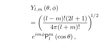
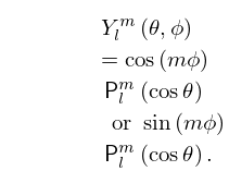
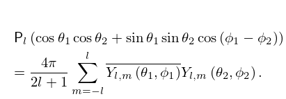
14: 14.30 Spherical and Spheroidal Harmonics
…
►
14.30.1
►
14.30.2
…
►See also (34.3.22), and for further related integrals see Askey et al. (1986).
…
►where and .
…
►
14.30.9
…
