complementary%20exponential%20integral
(0.005 seconds)
1—10 of 11 matching pages
1: 7.24 Approximations
Cody (1969) provides minimax rational approximations for and . The maximum relative precision is about 20S.
Cody et al. (1970) gives minimax rational approximations to Dawson’s integral (maximum relative precision 20S–22S).
Luke (1969b, pp. 323–324) covers and for (the Chebyshev coefficients are given to 20D); and for (the Chebyshev coefficients are given to 20D and 15D, respectively). Coefficients for the Fresnel integrals are given on pp. 328–330 (20D).
Shepherd and Laframboise (1981) gives coefficients of Chebyshev series for on (22D).
Luke (1969b, vol. 2, pp. 422–435) gives main diagonal Padé approximations for , , , , and ; approximate errors are given for a selection of -values.
2: 7.23 Tables
Abramowitz and Stegun (1964, Chapter 7) includes , , , 10D; , , 8S; , , 7D; , , , 6S; , , 10D; , , 9D; , , , 7D; , , , , 15D.
Abramowitz and Stegun (1964, Table 27.6) includes the Goodwin–Staton integral , , 4D; also , , 4D.
Zhang and Jin (1996, pp. 637, 639) includes , , , 8D; , , , 8D.
Zhang and Jin (1996, pp. 638, 640–641) includes the real and imaginary parts of , , , 7D and 8D, respectively; the real and imaginary parts of , , , 8D, together with the corresponding modulus and phase to 8D and 6D (degrees), respectively.
Fettis et al. (1973) gives the first 100 zeros of and (the table on page 406 of this reference is for , not for ), 11S.
3: 6.19 Tables
§6.19(ii) Real Variables
►Abramowitz and Stegun (1964, Chapter 5) includes , , , , ; , , , , ; , , , , ; , , , , ; , , . Accuracy varies but is within the range 8S–11S.
Zhang and Jin (1996, pp. 652, 689) includes , , , 8D; , , , 8S.
Abramowitz and Stegun (1964, Chapter 5) includes the real and imaginary parts of , , , 6D; , , , 6D; , , , 6D.
Zhang and Jin (1996, pp. 690–692) includes the real and imaginary parts of , , , 8S.
4: 6.20 Approximations
Cody and Thacher (1968) provides minimax rational approximations for , with accuracies up to 20S.
Cody and Thacher (1969) provides minimax rational approximations for , with accuracies up to 20S.
Luke (1969b, pp. 41–42) gives Chebyshev expansions of , , and for , . The coefficients are given in terms of series of Bessel functions.
Luke (1969b, pp. 321–322) covers and for (the Chebyshev coefficients are given to 20D); for (20D), and for (15D). Coefficients for the sine and cosine integrals are given on pp. 325–327.
Luke (1969b, pp. 411–414) gives rational approximations for .
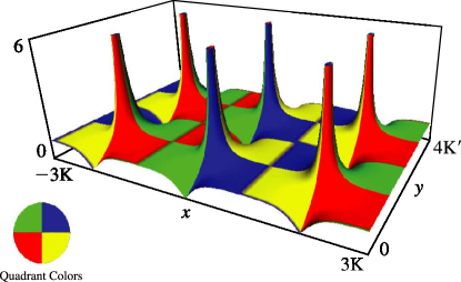
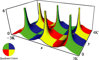
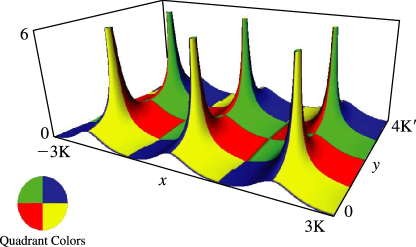
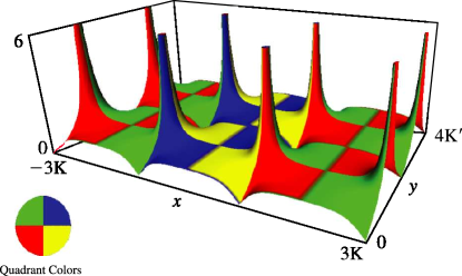
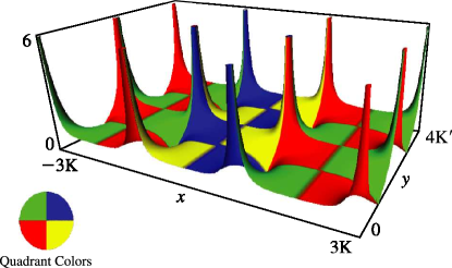
5: 22.3 Graphics
6: Bibliography F
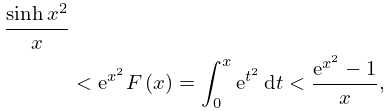
7: 7.8 Inequalities
§7.8 Inequalities
… ►8: Software Index
| Open Source | With Book | Commercial | |||||||||||||||||||||||
| … | |||||||||||||||||||||||||
| 6 Exponential, Logarithmic, Sine, and Cosine Integrals | |||||||||||||||||||||||||
| 6.21(ii) , , , , , , | ✓ | ✓ | ✓ | ✓ | ✓ | ✓ | ✓ | ✓ | ✓ | ✓ | ✓ | ✓ | ✓ | ✓ | ✓ | ✓ | ✓ | ✓ | ✓ | ✓ | ✓ | ✓ | |||
| … | |||||||||||||||||||||||||
| 7.25(ii) , , , | ✓ | ✓ | ✓ | ✓ | ✓ | ✓ | ✓ | ✓ | ✓ | ✓ | ✓ | ✓ | ✓ | ✓ | ✓ | ✓ | ✓ | ✓ | ✓ | ✓ | ✓ | NMS | |||
| … | |||||||||||||||||||||||||
| 8.28(vii) , | ✓ | ✓ | ✓ | ✓ | ✓ | ✓ | |||||||||||||||||||
| … | |||||||||||||||||||||||||
| 20 Theta Functions | |||||||||||||||||||||||||
| … | |||||||||||||||||||||||||
9: Errata
Originally, a factor of was missing from the terms containing the .
Reported by Fred Hucht on 2020-08-06
