Gauss%E2%80%93Laguerre%20formula

♦ 11—20 of 391 matching pages ♦

(0.003 seconds)

11—20 of 391 matching pages

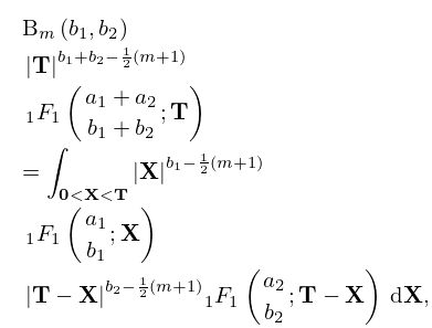
11: 35.8 Generalized Hypergeometric Functions of Matrix Argument

… ►

§35.8(iii) ${{}_{3}F_{2}}$ Case

►

Kummer Transformation

… ►

Pfaff–Saalschütz Formula

… ►

Thomae Transformation

… ►Multidimensional Mellin–Barnes integrals are established in Ding et al. (1996) for the functions

{{}_{p}F_{q}}

and

{{}_{p+1}F_{p}}

of matrix argument. …

12: Bibliography K

… ►

K. W. J. Kadell (1994) A proof of the

q

-Macdonald-Morris conjecture for

BC_{n}

. Mem. Amer. Math. Soc. 108 (516), pp. vi+80.

ⓘ

External Links:: ISSN 0065-9266, MathReview (Eric M. Opdam), ZentralBlatt
Referenced by:: §17.14.
Encodings:: BibTeX

… ►

S. L. Kalla (1992) On the evaluation of the Gauss hypergeometric function. C. R. Acad. Bulgare Sci. 45 (6), pp. 35–36.

ⓘ

External Links:: ISSN 0861-1459, MathReview, ZentralBlatt
Referenced by:: §15.15, §15.19(i).
Encodings:: BibTeX

… ►

E. H. Kaufman and T. D. Lenker (1986) Linear convergence and the bisection algorithm. Amer. Math. Monthly 93 (1), pp. 48–51.

ⓘ

External Links:: ISSN 0002-9890, FullText, MathReview (J. G. Herriot), ZentralBlatt
Referenced by:: §3.8(iii).
Encodings:: BibTeX

… ►

A. V. Kitaev and A. H. Vartanian (2004) Connection formulae for asymptotics of solutions of the degenerate third Painlevé equation. I. Inverse Problems 20 (4), pp. 1165–1206.

ⓘ

External Links:: ISSN 0266-5611, Document, MathReview (Shun Shimomura), ZentralBlatt
Referenced by:: §32.11(iv).
Encodings:: BibTeX

… ►

T. H. Koornwinder (1977) The addition formula for Laguerre polynomials. SIAM J. Math. Anal. 8 (3), pp. 535–540.

ⓘ

External Links:: Document, MathReview (M. Mikolas), ZentralBlatt
Referenced by:: (18.14.8), §18.14(i), §18.17(ii), §18.18(ii).
Encodings:: BibTeX

…

13: Bibliography

… ►

G. Almkvist and B. Berndt (1988) Gauss, Landen, Ramanujan, the arithmetic-geometric mean, ellipses,

\pi

, and the Ladies Diary. Amer. Math. Monthly 95 (7), pp. 585–608.

ⓘ

External Links:: ISSN 0002-9890, FullText, Document, MathReview (R. A. Askey), ZentralBlatt
Referenced by:: §19.9(i).
Encodings:: BibTeX

… ►

D. E. Amos, S. L. Daniel, and M. K. Weston (1977) Algorithm 511: CDC 6600 subroutines IBESS and JBESS for Bessel functions

I_{\nu}(x)

and

J_{\nu}(x)

x\geq 0

\nu\geq 0

. ACM Trans. Math. Software 3 (1), pp. 93–95.

ⓘ

Notes:: Single-precision Fortran, maximum accuracy 16S.
External Links:: ISSN 0098-3500, Document, Companion paper. Erratum. GAMS (module 511; package TOMS)
Referenced by:: 1st item, 1st item.
Encodings:: BibTeX

… ►

D. E. Amos (1990) Algorithm 683: A portable FORTRAN subroutine for exponential integrals of a complex argument. ACM Trans. Math. Software 16 (2), pp. 178–182.

ⓘ

Notes:: Double- and single-precision Fortran, maximum accuracy 18S or 14S.
External Links:: ISSN 0098-3500, Document, GAMS (module 683; package TOMS), MathReview, ZentralBlatt
Referenced by:: 1st item, 1st item.
Encodings:: BibTeX

… ►

G. E. Andrews, R. Askey, and R. Roy (1999) Special Functions. Encyclopedia of Mathematics and its Applications, Vol. 71, Cambridge University Press, Cambridge.

ⓘ

External Links:: ISBN 0-521-62321-9, MathReview (Bruce C. Berndt), ZentralBlatt
Referenced by:: §1.10(vii), §1.15(iii), §1.15(vi), §1.15(vii), §10.22(vi), §13.6(v), §13.9(i), Ch.13, §14.3(iii), §14.30(iv), §15.10(i), §15.11(i), §15.11(ii), §15.14, §15.17(iv), §15.2(i), §15.4(ii), §15.5(i), §15.5(ii), §15.6, §15.7, §15.8(iv), §15.8(iii), Ch.15, §16.4(ii), §16.4(iii), §16.4(v), §16.4(v), Ch.16, §17.12, Ch.17, §18.10(ii), §18.10(iv), §18.11(i), §18.12, (18.17.41_5), §18.17(iv), §18.17(viii), §18.18(iv), §18.18(iv), §18.18(v), §18.18(vii), §18.2(i), §18.2(iv), §18.2(vi), §18.20(ii), §18.22(i), §18.25(ii), §18.26(i), Table 18.3.1, §18.38(ii), §18.5(iii), (18.7.25), Ch.18, §26.19, §4.10(i), §4.10(ii), §5.13, §5.14, §5.16, §5.16, §5.18(i), §5.18(ii), §5.18(iii), §5.20, §5.4(ii), §5.5(iv), Ch.5, Ch.6, Profile Richard A. Askey, Profile Ranjan Roy, Erratum (V1.0.28) for Table 18.3.1.
Encodings:: BibTeX

… ►

M. J. Atia, A. Martínez-Finkelshtein, P. Martínez-González, and F. Thabet (2014) Quadratic differentials and asymptotics of Laguerre polynomials with varying complex parameters. J. Math. Anal. Appl. 416 (1), pp. 52–80.

ⓘ

External Links:: ISSN 0022-247X, Document, Link, MathReview (Vivek Sahai), ZentralBlatt
Referenced by:: §18.15(vi), §18.15(vi).
Encodings:: BibTeX

…

14: 15.9 Relations to Other Functions

… ►

15.9.2

C^{(\lambda)}_{n}\left(x\right)=\frac{{\left(2\lambda\right)_{n}}}{n!}F\left({% -n,n+2\lambda\atop\lambda+\frac{1}{2}};\frac{1-x}{2}\right).

ⓘ

Symbols:: $F\left(\NVar{a},\NVar{b};\NVar{c};\NVar{z}\right)$ or $F\left({\NVar{a},\NVar{b}\atop\NVar{c}};\NVar{z}\right)$ : $={{}_{2}F_{1}}\left(\NVar{a},\NVar{b};\NVar{c};\NVar{z}\right)$ Gauss’ hypergeometric function, ${\left(\NVar{a}\right)_{\NVar{n}}}$ : Pochhammer’s symbol (or shifted factorial), $!$ : factorial (as in $n!$ ), $C^{(\NVar{\lambda})}_{\NVar{n}}\left(\NVar{x}\right)$ : ultraspherical (or Gegenbauer) polynomial, $x$ : real variable and $n$ : integer
Permalink:: http://dlmf.nist.gov/15.9.E2
Encodings:: pMML, png, TeX
See also:: Annotations for §15.9(i), §15.9(i), §15.9 and Ch.15

►

15.9.3

C^{(\lambda)}_{n}\left(x\right)=(2x)^{n}\frac{{\left(\lambda\right)_{n}}}{n!}F% \left({-\frac{1}{2}n,\frac{1}{2}(1-n)\atop 1-\lambda-n};\frac{1}{x^{2}}\right).

ⓘ

Symbols:: $F\left(\NVar{a},\NVar{b};\NVar{c};\NVar{z}\right)$ or $F\left({\NVar{a},\NVar{b}\atop\NVar{c}};\NVar{z}\right)$ : $={{}_{2}F_{1}}\left(\NVar{a},\NVar{b};\NVar{c};\NVar{z}\right)$ Gauss’ hypergeometric function, ${\left(\NVar{a}\right)_{\NVar{n}}}$ : Pochhammer’s symbol (or shifted factorial), $!$ : factorial (as in $n!$ ), $C^{(\NVar{\lambda})}_{\NVar{n}}\left(\NVar{x}\right)$ : ultraspherical (or Gegenbauer) polynomial, $x$ : real variable and $n$ : integer
Permalink:: http://dlmf.nist.gov/15.9.E3
Encodings:: pMML, png, TeX
See also:: Annotations for §15.9(i), §15.9(i), §15.9 and Ch.15

… ►

15.9.5

T_{n}\left(x\right)=F\left({-n,n\atop\frac{1}{2}};\frac{1-x}{2}\right).

ⓘ

Symbols:: $T_{\NVar{n}}\left(\NVar{x}\right)$ : Chebyshev polynomial of the first kind, $F\left(\NVar{a},\NVar{b};\NVar{c};\NVar{z}\right)$ or $F\left({\NVar{a},\NVar{b}\atop\NVar{c}};\NVar{z}\right)$ : $={{}_{2}F_{1}}\left(\NVar{a},\NVar{b};\NVar{c};\NVar{z}\right)$ Gauss’ hypergeometric function, $x$ : real variable and $n$ : integer
Permalink:: http://dlmf.nist.gov/15.9.E5
Encodings:: pMML, png, TeX
See also:: Annotations for §15.9(i), §15.9(i), §15.9 and Ch.15

… ►

15.9.7

P_{n}\left(x\right)=F\left({-n,n+1\atop 1};\frac{1-x}{2}\right).

ⓘ

Symbols:: $F\left(\NVar{a},\NVar{b};\NVar{c};\NVar{z}\right)$ or $F\left({\NVar{a},\NVar{b}\atop\NVar{c}};\NVar{z}\right)$ : $={{}_{2}F_{1}}\left(\NVar{a},\NVar{b};\NVar{c};\NVar{z}\right)$ Gauss’ hypergeometric function, $P_{\NVar{n}}\left(\NVar{x}\right)$ : Legendre polynomial, $x$ : real variable and $n$ : integer
Permalink:: http://dlmf.nist.gov/15.9.E7
Encodings:: pMML, png, TeX
See also:: Annotations for §15.9(i), §15.9(i), §15.9 and Ch.15

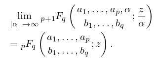
… ►The following formulas apply with principal branches of the hypergeometric functions, associated Legendre functions, and fractional powers. …

15: 31.7 Relations to Other Functions

… ►

§31.7(i) Reductions to the Gauss Hypergeometric Function

… ►Other reductions of

\mathit{H\!\ell}

to a

{{}_{2}F_{1}}

, with at least one free parameter, exist iff the pair

(a,p)

takes one of a finite number of values, where

q=\alpha\beta p

. … ►

31.7.2

\mathit{H\!\ell}\left(2,\alpha\beta;\alpha,\beta,\gamma,\alpha+\beta-2\gamma+1% ;z\right)={{}_{2}F_{1}}\left(\tfrac{1}{2}\alpha,\tfrac{1}{2}\beta;\gamma;1-(1-% z)^{2}\right),

ⓘ

Symbols:: ${{}_{2}F_{1}}\left(\NVar{a},\NVar{b};\NVar{c};\NVar{z}\right)$ : $=F\left(\NVar{a},\NVar{b};\NVar{c};\NVar{z}\right)$ notation for Gauss’ hypergeometric function, $\mathit{H\!\ell}\left(\NVar{a},\NVar{q};\NVar{\alpha},\NVar{\beta},\NVar{% \gamma},\NVar{\delta};\NVar{z}\right)$ : Heun functions, $z$ : complex variable, $\gamma$ : real or complex parameter, $\alpha$ : real or complex parameter and $\beta$ : real or complex parameter
Permalink:: http://dlmf.nist.gov/31.7.E2
Encodings:: pMML, png, TeX
See also:: Annotations for §31.7(i), §31.7 and Ch.31

►

31.7.3

\mathit{H\!\ell}\left(4,\alpha\beta;\alpha,\beta,\tfrac{1}{2},\tfrac{2}{3}(% \alpha+\beta);z\right)={{}_{2}F_{1}}\left(\tfrac{1}{3}\alpha,\tfrac{1}{3}\beta% ;\tfrac{1}{2};1-(1-z)^{2}(1-\tfrac{1}{4}z)\right),

ⓘ

Symbols:: ${{}_{2}F_{1}}\left(\NVar{a},\NVar{b};\NVar{c};\NVar{z}\right)$ : $=F\left(\NVar{a},\NVar{b};\NVar{c};\NVar{z}\right)$ notation for Gauss’ hypergeometric function, $\mathit{H\!\ell}\left(\NVar{a},\NVar{q};\NVar{\alpha},\NVar{\beta},\NVar{% \gamma},\NVar{\delta};\NVar{z}\right)$ : Heun functions, $z$ : complex variable, $\alpha$ : real or complex parameter and $\beta$ : real or complex parameter
Permalink:: http://dlmf.nist.gov/31.7.E3
Encodings:: pMML, png, TeX
See also:: Annotations for §31.7(i), §31.7 and Ch.31

… ►Similar specializations of formulas in §31.3(ii) yield solutions in the neighborhoods of the singularities

\zeta=K

K+i{K^{\prime}}

, and

i{K^{\prime}}

, where

K

and

{K^{\prime}}

are related to

k

as in §19.2(ii).

16: 20.11 Generalizations and Analogs

… ►

§20.11(i) Gauss Sum

►For relatively prime integers

m, n

with

n>0

and

m n

even, the Gauss sum

G(m,n)

is defined by … … ► … ►Similar identities can be constructed for

{{}_{2}F_{1}}\left(\tfrac{1}{3},\tfrac{2}{3};1;k^{2}\right)

{{}_{2}F_{1}}\left(\tfrac{1}{4},\tfrac{3}{4};1;k^{2}\right)

, and

{{}_{2}F_{1}}\left(\tfrac{1}{6},\tfrac{5}{6};1;k^{2}\right)

. …

17: 16.8 Differential Equations

… ►the function

w={{}_{p}F_{q}}\left(\mathbf{a};\mathbf{b};z\right)

satisfies the differential equation … ►

w_{0}(z)={{}_{p}F_{q}}\left({a_{1},\dots,a_{p}\atop b_{1},\dots,b_{q}};z\right),

… ►We have the connection formula … ►Analytical continuation formulas for

{{}_{q+1}F_{q}}\left(\mathbf{a};\mathbf{b};z\right)

near

z=1

are given in Bühring (1987b) for the case

q=2

, and in Bühring (1992) for the general case. … ►

16.8.10

\lim_{|\alpha|\to\infty}{{}_{p+1}F_{q}}\left({a_{1},\dots,a_{p},\alpha\atop b_% {1},\dots,b_{q}};\frac{z}{\alpha}\right)={{}_{p}F_{q}}\left({a_{1},\dots,a_{p}% \atop b_{1},\dots,b_{q}};z\right).

ⓘ

Symbols:: ${{}_{\NVar{p}}F_{\NVar{q}}}\left(\NVar{a_{1},\dots,a_{p}};\NVar{b_{1},\dots,b_% {q}};\NVar{z}\right)$ or ${{}_{\NVar{p}}F_{\NVar{q}}}\left({\NVar{a_{1},\dots,a_{p}}\atop\NVar{b_{1},% \dots,b_{q}}};\NVar{z}\right)$ : alternatively ${{}_{\NVar{p}}F_{\NVar{q}}}\left(\NVar{\mathbf{a}};\NVar{\mathbf{b}};\NVar{z}\right)$ or ${{}_{\NVar{p}}F_{\NVar{q}}}\left({\NVar{\mathbf{a}}\atop\NVar{\mathbf{b}}};% \NVar{z}\right)$
generalized hypergeometric function, $p$ : nonnegative integer, $q$ : nonnegative integer, $z$ : complex variable, $a,a_{1},\ldots,a_{p}$ : real or complex parameters and $b,b_{1},\ldots,b_{q}$ : real or complex parameters
Permalink:: http://dlmf.nist.gov/16.8.E10
Encodings:: pMML, png, TeX
See also:: Annotations for §16.8(iii), §16.8 and Ch.16

…

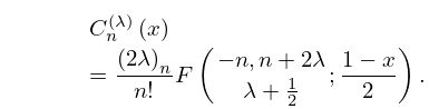
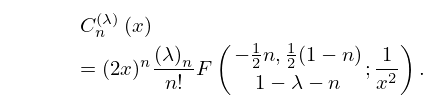
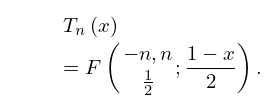
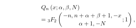
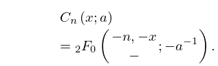
18: 18.20 Hahn Class: Explicit Representations

… ►

§18.20(i) Rodrigues Formulas

… ►

18.20.5

Q_{n}\left(x;\alpha,\beta,N\right)={{}_{3}F_{2}}\left({-n,n+\alpha+\beta+1,-x% \atop\alpha+1,-N};1\right),

n=0,1,\dots,N

ⓘ

Symbols:: ${{}_{\NVar{p}}F_{\NVar{q}}}\left(\NVar{a_{1},\dots,a_{p}};\NVar{b_{1},\dots,b_% {q}};\NVar{z}\right)$ or ${{}_{\NVar{p}}F_{\NVar{q}}}\left({\NVar{a_{1},\dots,a_{p}}\atop\NVar{b_{1},% \dots,b_{q}}};\NVar{z}\right)$ : alternatively ${{}_{\NVar{p}}F_{\NVar{q}}}\left(\NVar{\mathbf{a}};\NVar{\mathbf{b}};\NVar{z}\right)$ or ${{}_{\NVar{p}}F_{\NVar{q}}}\left({\NVar{\mathbf{a}}\atop\NVar{\mathbf{b}}};% \NVar{z}\right)$
generalized hypergeometric function, $Q_{\NVar{n}}\left(\NVar{x};\NVar{\alpha},\NVar{\beta},\NVar{N}\right)$ : Hahn polynomial, $N$ : positive integer, $n$ : nonnegative integer and $x$ : real variable
Referenced by:: §18.20(ii), §18.21(ii), §18.23, §18.26(ii), §18.27(ii), §18.38(iii)
Permalink:: http://dlmf.nist.gov/18.20.E5
Encodings:: pMML, png, TeX
See also:: Annotations for §18.20(ii), §18.20 and Ch.18

►

18.20.6

K_{n}\left(x;p,N\right)={{}_{2}F_{1}}\left({-n,-x\atop-N};p^{-1}\right),

n=0,1,\dots,N

ⓘ

Symbols:: ${{}_{2}F_{1}}\left(\NVar{a},\NVar{b};\NVar{c};\NVar{z}\right)$ : $=F\left(\NVar{a},\NVar{b};\NVar{c};\NVar{z}\right)$ notation for Gauss’ hypergeometric function, $K_{\NVar{n}}\left(\NVar{x};\NVar{p},\NVar{N}\right)$ : Krawtchouk polynomial, $N$ : positive integer, $n$ : nonnegative integer and $x$ : real variable
Referenced by:: §18.19, §18.21(ii)
Permalink:: http://dlmf.nist.gov/18.20.E6
Encodings:: pMML, png, TeX
See also:: Annotations for §18.20(ii), §18.20 and Ch.18

►

18.20.7

M_{n}\left(x;\beta,c\right)={{}_{2}F_{1}}\left({-n,-x\atop\beta};1-c^{-1}% \right).

ⓘ

Symbols:: ${{}_{2}F_{1}}\left(\NVar{a},\NVar{b};\NVar{c};\NVar{z}\right)$ : $=F\left(\NVar{a},\NVar{b};\NVar{c};\NVar{z}\right)$ notation for Gauss’ hypergeometric function, $M_{\NVar{n}}\left(\NVar{x};\NVar{\beta},\NVar{c}\right)$ : Meixner polynomial, $n$ : nonnegative integer and $x$ : real variable
Referenced by:: §18.21(ii), §18.26(ii)
Permalink:: http://dlmf.nist.gov/18.20.E7
Encodings:: pMML, png, TeX
See also:: Annotations for §18.20(ii), §18.20 and Ch.18

►

18.20.8

C_{n}\left(x;a\right)={{}_{2}F_{0}}\left({-n,-x\atop-};-a^{-1}\right).

ⓘ

Symbols:: $C_{\NVar{n}}\left(\NVar{x};\NVar{a}\right)$ : Charlier polynomial, ${{}_{\NVar{p}}F_{\NVar{q}}}\left(\NVar{a_{1},\dots,a_{p}};\NVar{b_{1},\dots,b_% {q}};\NVar{z}\right)$ or ${{}_{\NVar{p}}F_{\NVar{q}}}\left({\NVar{a_{1},\dots,a_{p}}\atop\NVar{b_{1},% \dots,b_{q}}};\NVar{z}\right)$ : alternatively ${{}_{\NVar{p}}F_{\NVar{q}}}\left(\NVar{\mathbf{a}};\NVar{\mathbf{b}};\NVar{z}\right)$ or ${{}_{\NVar{p}}F_{\NVar{q}}}\left({\NVar{\mathbf{a}}\atop\NVar{\mathbf{b}}};% \NVar{z}\right)$
generalized hypergeometric function, $n$ : nonnegative integer and $x$ : real variable
Referenced by:: §13.6(v), §18.19, §18.20(ii), §18.21(ii)
Permalink:: http://dlmf.nist.gov/18.20.E8
Encodings:: pMML, png, TeX
See also:: Annotations for §18.20(ii), §18.20 and Ch.18

…

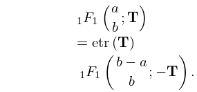
19: 35.7 Gaussian Hypergeometric Function of Matrix Argument

… ►

Gauss Formula

… ►

Reflection Formula

… ►Subject to the conditions (a)–(c), the function

f(\mathbf{T})={{}_{2}F_{1}}\left(a,b;c;\mathbf{T}\right)

is the unique solution of each partial differential equation … ►Systems of partial differential equations for the

{{}_{0}F_{1}}

(defined in §35.8) and

{{}_{1}F_{1}}

functions of matrix argument can be obtained by applying (35.8.9) and (35.8.10) to (35.7.9). … ►

35.7.10

{{}_{2}F_{1}}\left({\alpha a,\alpha b\atop\alpha c};\mathbf{T}\right)

ⓘ

Symbols:: ${{}_{\NVar{p}}F_{\NVar{q}}}\left(\NVar{a_{1},\dots,a_{p}};\NVar{b_{1},\dots,b_% {q}};\NVar{\mathbf{T}}\right)$ or ${{}_{\NVar{p}}F_{\NVar{q}}}\left({\NVar{a_{1},\dots,a_{p}}\atop\NVar{b_{1},% \dots,b_{q}}};\NVar{\mathbf{T}}\right)$ : generalized hypergeometric function of matrix argument, $a$ : complex variable, $\mathbf{T}$ : real symmetric $m\times m$ matrix, $b$ : complex variable, $c$ : complex variable and $\alpha\to\infty$ : parameter
Permalink:: http://dlmf.nist.gov/35.7.E10
Encodings:: pMML, png, TeX
See also:: Annotations for §35.7(iv), §35.7 and Ch.35

…

20: 35.6 Confluent Hypergeometric Functions of Matrix Argument

… ►

Laguerre Form

►

35.6.3

L^{(\gamma)}_{\nu}\left(\mathbf{T}\right)=\frac{\Gamma_{m}\left(\gamma+\nu+% \frac{1}{2}(m+1)\right)}{\Gamma_{m}\left(\gamma+\frac{1}{2}(m+1)\right)}\*{{}_% {1}F_{1}}\left({-\nu\atop\gamma+\frac{1}{2}(m+1)};\mathbf{T}\right),

\Re\left(\gamma\right),\Re\left(\gamma+\nu\right)>-1

ⓘ

Defines:: $L^{(\NVar{\gamma})}_{\NVar{\nu}}\left(\NVar{\mathbf{T}}\right)$ : Laguerre function of matrix argument
Symbols:: ${{}_{\NVar{p}}F_{\NVar{q}}}\left(\NVar{a_{1},\dots,a_{p}};\NVar{b_{1},\dots,b_% {q}};\NVar{\mathbf{T}}\right)$ or ${{}_{\NVar{p}}F_{\NVar{q}}}\left({\NVar{a_{1},\dots,a_{p}}\atop\NVar{b_{1},% \dots,b_{q}}};\NVar{\mathbf{T}}\right)$ : generalized hypergeometric function of matrix argument, $\Gamma_{\NVar{m}}\left(\NVar{a}\right)$ : multivariate gamma function, $\Re$ : real part, $\mathbf{T}$ : real symmetric $m\times m$ matrix and $m$ : positive integer
Permalink:: http://dlmf.nist.gov/35.6.E3
Encodings:: pMML, png, TeX
See also:: Annotations for §35.6(i), §35.6(i), §35.6 and Ch.35

… ►

35.6.6

\mathrm{B}_{m}\left(b_{1},b_{2}\right)\left|\mathbf{T}\right|^{b_{1}+b_{2}-% \frac{1}{2}(m+1)}{{}_{1}F_{1}}\left({a_{1}+a_{2}\atop b_{1}+b_{2}};\mathbf{T}% \right)=\int_{\boldsymbol{{0}}<\mathbf{X}<\mathbf{T}}\left|\mathbf{X}\right|^{% b_{1}-\frac{1}{2}(m+1)}{{}_{1}F_{1}}\left({a_{1}\atop b_{1}};\mathbf{X}\right)% {\left|\mathbf{T}-\mathbf{X}\right|}^{b_{2}-\frac{1}{2}(m+1)}{{}_{1}F_{1}}% \left({a_{2}\atop b_{2}};\mathbf{T}-\mathbf{X}\right)\,\mathrm{d}{\mathbf{X}},

\Re\left(b_{1}\right),\Re\left(b_{2}\right)>\frac{1}{2}(m-1)

►

35.6.7

{{}_{1}F_{1}}\left({a\atop b};\mathbf{T}\right)=\operatorname{etr}\left(% \mathbf{T}\right){{}_{1}F_{1}}\left({b-a\atop b};-\mathbf{T}\right).

ⓘ

Symbols:: ${{}_{\NVar{p}}F_{\NVar{q}}}\left(\NVar{a_{1},\dots,a_{p}};\NVar{b_{1},\dots,b_% {q}};\NVar{\mathbf{T}}\right)$ or ${{}_{\NVar{p}}F_{\NVar{q}}}\left({\NVar{a_{1},\dots,a_{p}}\atop\NVar{b_{1},% \dots,b_{q}}};\NVar{\mathbf{T}}\right)$ : generalized hypergeometric function of matrix argument, $\operatorname{etr}\left(\NVar{\mathbf{A}}\right)$ : exponential of trace, $a$ : complex variable, $\mathbf{T}$ : real symmetric $m\times m$ matrix and $b$ : complex variable
Permalink:: http://dlmf.nist.gov/35.6.E7
Encodings:: pMML, png, TeX
See also:: Annotations for §35.6(ii), §35.6 and Ch.35

… ►

35.6.9

\lim_{a\to\infty}{{}_{1}F_{1}}\left({a\atop\nu+\frac{1}{2}(m+1)};-a^{-1}% \mathbf{T}\right)=\frac{A_{\nu}\left(\mathbf{T}\right)}{A_{\nu}\left(% \boldsymbol{{0}}\right)}.

ⓘ

Symbols:: $A_{\NVar{\nu}}\left(\NVar{\mathbf{T}}\right)$ : Bessel function of matrix argument (first kind), ${{}_{\NVar{p}}F_{\NVar{q}}}\left(\NVar{a_{1},\dots,a_{p}};\NVar{b_{1},\dots,b_% {q}};\NVar{\mathbf{T}}\right)$ or ${{}_{\NVar{p}}F_{\NVar{q}}}\left({\NVar{a_{1},\dots,a_{p}}\atop\NVar{b_{1},% \dots,b_{q}}};\NVar{\mathbf{T}}\right)$ : generalized hypergeometric function of matrix argument, $a$ : complex variable, $\mathbf{T}$ : real symmetric $m\times m$ matrix, $m$ : positive integer and $\boldsymbol{{0}}$ : $m\times m$ matrix of zeros
Permalink:: http://dlmf.nist.gov/35.6.E9
Encodings:: pMML, png, TeX
See also:: Annotations for §35.6(iii), §35.6 and Ch.35

…