.奥乔亚世界杯扑救『网址:mxsty.cc』.世界杯亚运会.m4x5s2-2022年11月29日4时50分10秒eosssivzt
(0.001 seconds)
31—40 of 241 matching pages
31: 7.23 Tables
Abramowitz and Stegun (1964, Chapter 7) includes , , , 10D; , , 8S; , , 7D; , , , 6S; , , 10D; , , 9D; , , , 7D; , , , , 15D.
Zhang and Jin (1996, pp. 637, 639) includes , , , 8D; , , , 8D.
Fettis et al. (1973) gives the first 100 zeros of and (the table on page 406 of this reference is for , not for ), 11S.
Zhang and Jin (1996, p. 642) includes the first 10 zeros of , 9D; the first 25 distinct zeros of and , 8S.
32: Bibliography W
33: Bibliography F
34: 8.26 Tables
Pearson (1968) tabulates for , , with , to 7D.
Zhang and Jin (1996, Table 3.9) tabulates for , , to 8D.
Pagurova (1961) tabulates for , to 4-9S; for , to 7D; for , to 7S or 7D.
Stankiewicz (1968) tabulates for , to 7D.
Zhang and Jin (1996, Table 19.1) tabulates for , to 7D or 8S.
35: 5.22 Tables
36: Bibliography S
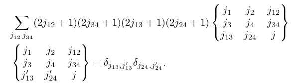
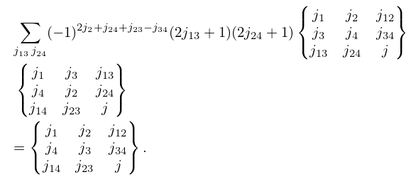
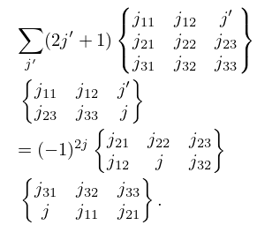
37: 34.7 Basic Properties: Symbol
38: 6.19 Tables
Abramowitz and Stegun (1964, Chapter 5) includes , , , , ; , , , , ; , , , , ; , , , , ; , , . Accuracy varies but is within the range 8S–11S.
Zhang and Jin (1996, pp. 690–692) includes the real and imaginary parts of , , , 8S.
