.%E7%94%B7%E7%AF%AE%E4%B8%96%E7%95%8C%E6%9D%AF%E9%A2%84%E9%80%89%E8%B5%9B%E4%B8%AD%E5%9B%BDvs%E9%BB%8E%E5%B7%B4%E5%AB%A9%E3%80%8Ewn4.com%E3%80%8F%E5%92%AA%E5%92%95%E4%B8%96%E7%95%8C%E6%9D%AF%E8%90%A5%E9%94%80%E6%96%B9%E6%A1%88.w6n2c9o.2022%E5%B9%B411%E6%9C%8829%E6%97%A55%E6%97%B652%E5%88%862%E7%A7%92.yeyo8yaka

SearchAdvancedHelp

(0.021 seconds)

21—30 of 666 matching pages

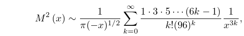
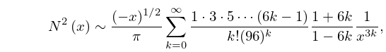
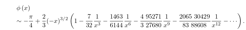
21: 33.20 Expansions for Small $|ϵ|$

… ►where ►

33.20.4 $${𝖥}_k(\mathrm{\ell };r)=\sum _{p=2k}^{3k}{(2r)}^{(p+1)/2}{C}_{k,p}{J}_{2\mathrm{\ell }+1+p}\left(\sqrt{8r}\right),$$ $r>0$,

ⓘ

Symbols:

$J_{\nu }\left(z\right)$: Bessel function of the first kind, $k$: nonnegative integer, $\mathrm{\ell }$: nonnegative integer, $r$: real variable, ${𝖥}_k(\mathrm{\ell };r)$: coefficient and $C_{k,p}$: coefficients

Permalink:

http://dlmf.nist.gov/33.20.E4

Encodings:

pMML, png, TeX

See also:

Annotations for §33.20(ii), §33.20 and Ch.33

►

33.20.5 $${𝖥}_k(\mathrm{\ell };r)=\sum _{p=2k}^{3k}{(-1)}^{\mathrm{\ell }+1+p}{(2|r|)}^{(p+1)/2}{C}_{k,p}{I}_{2\mathrm{\ell }+1+p}\left(\sqrt{8|r|}\right),$$ .

ⓘ

Symbols:

$I_{\nu }\left(z\right)$: modified Bessel function of the first kind, $k$: nonnegative integer, $\mathrm{\ell }$: nonnegative integer, $r$: real variable, ${𝖥}_k(\mathrm{\ell };r)$: coefficient and $C_{k,p}$: coefficients

Permalink:

http://dlmf.nist.gov/33.20.E5

Encodings:

pMML, png, TeX

See also:

Annotations for §33.20(ii), §33.20 and Ch.33

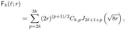
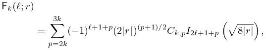
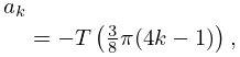
►The functions $J$ and $I$ are as in §§10.2(ii), 10.25(ii), and the coefficients $C_{k,p}$ are given by $C_{0,0}=1$, $C_{1,0}=0$, and … ►The functions $Y$ and $K$ are as in §§10.2(ii), 10.25(ii), and the coefficients $C_{k,p}$ are given by (33.20.6). …

22: 6.14 Integrals

… ►

6.14.1 $${\int }_0^{\mathrm{\infty }}{\mathrm{e}}^{-at}{E}_1\left(t\right)dt=\frac{1}{a}\ln \left(1+a\right),$$ $\mathrm{\Re }a>-1$,

ⓘ

Symbols:

$dx$: differential of $x$ , $\mathrm{e}$: base of natural logarithm, $E_1\left(z\right)$: exponential integral, $\int$: integral, $\ln z$: principal branch of logarithm function and $\mathrm{\Re }$: real part

A&S Ref:

5.1.34 (special case of)

Permalink:

http://dlmf.nist.gov/6.14.E1

Encodings:

pMML, png, TeX

See also:

Annotations for §6.14(i), §6.14 and Ch.6

… ►

6.14.4 $${\int }_0^{\mathrm{\infty }}{E}_1^2\left(t\right)dt=2\ln 2,$$

ⓘ

Symbols:

$dx$: differential of $x$ , $E_1\left(z\right)$: exponential integral, $\int$: integral and $\ln z$: principal branch of logarithm function

A&S Ref:

5.1.33

Permalink:

http://dlmf.nist.gov/6.14.E4

Encodings:

pMML, png, TeX

See also:

Annotations for §6.14(ii), §6.14 and Ch.6

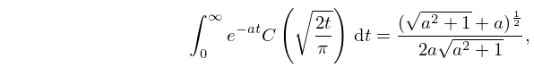
… ►For collections of integrals, see Apelblat (1983, pp. 110–123), Bierens de Haan (1939, pp. 373–374, 409, 479, 571–572, 637, 664–673, 680–682, 685–697), Erdélyi et al. (1954a, vol. 1, pp. 40–42, 96–98, 177–178, 325), Geller and Ng (1969), Gradshteyn and Ryzhik (2000, §§5.2–5.3 and 6.2–6.27), Marichev (1983, pp. 182–184), Nielsen (1906b), Oberhettinger (1974, pp. 139–141), Oberhettinger (1990, pp. 53–55 and 158–160), Oberhettinger and Badii (1973, pp. 172–179), Prudnikov et al. (1986b, vol. 2, pp. 24–29 and 64–92), Prudnikov et al. (1992a, §§3.4–3.6), Prudnikov et al. (1992b, §§3.4–3.6), and Watrasiewicz (1967).

23: Bibliography M

… ►

Inequalities for the zeros of Bessel functions. SIAM J. Math. Anal. 8 (1), pp. 166–170.

ⓘ

External Links:

ISSN 1095-7154, Document, MathReview (Mary L. Boas), ZentralBlatt

Referenced by:

§10.21(iv).

Encodings:

BibTeX

… ►

Calculation of the modified Bessel functions of the second kind with complex argument. Math. Comp. 20 (95), pp. 407–412.

ⓘ

External Links:

ISSN 0025-5718, FullText, MathReview (H. E. Fettis), ZentralBlatt

Referenced by:

§10.74(iii).

Encodings:

BibTeX

… ►

Algorithm 149: Complete elliptic integral. Comm. ACM 5 (12), pp. 605.

ⓘ

Notes:

Includes Algol program, maximum accuracy 10D. For remark see ACM Trans. Math. Software 4 (1978), p. 95

External Links:

ISSN 0001-0782, Document

Referenced by:

§19.39(ii).

Encodings:

BibTeX

… ►

Hierarchies and logarithmic oscillations in the temporal relaxation patterns of proteins and other complex systems. Proc. Nat. Acad. Sci. U .S. A. 96 (20), pp. 11085–11089.

ⓘ

External Links:

FullText

Referenced by:

§8.24(i).

Encodings:

BibTeX

… ►

Lattice Statistics. In Applied Combinatorial Mathematics, E. F. Beckenbach (Ed.), University of California Engineering and Physical Sciences Extension Series, pp. 96–143.

ⓘ

Notes:

Reprinted by Robert E. Krieger Publishing Co. in 1981.

External Links:

ZentralBlatt

Referenced by:

§26.20.

Encodings:

BibTeX

…

24: 5.13 Integrals

…

25: 27.2 Functions

… ►

27.2.9 $$d\left(n\right)=\sum _{d|n}1$$

ⓘ

Symbols:

$d_k\left(n\right)$: divisor function, $d$: positive integer and $n$: positive integer

A&S Ref:

24.3.3 I.A

Permalink:

http://dlmf.nist.gov/27.2.E9

Encodings:

pMML, png, TeX

See also:

Annotations for §27.2(i), §27.2 and Ch.27

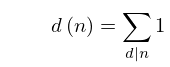
… ►It is the special case $k=2$ of the function $d_k\left(n\right)$ that counts the number of ways of expressing $n$ as the product of $k$ factors, with the order of factors taken into account. …Note that ${\sigma }_0\left(n\right)=d\left(n\right)$. … ►Table 27.2.2 tabulates the Euler totient function $\varphi \left(n\right)$, the divisor function $d\left(n\right)$ ($={\sigma }_0(n)$), and the sum of the divisors $\sigma (n)$ ($={\sigma }_1(n)$), for $n=1(1)52$. … ►

Table 27.2.2: Functions related to division.

► ►►►

$n$	$\varphi \left(n\right)$	$d\left(n\right)$	$\sigma \left(n\right)$	$n$	$\varphi \left(n\right)$	$d\left(n\right)$	$\sigma \left(n\right)$	$n$	$\varphi \left(n\right)$	$d\left(n\right)$	$\sigma \left(n\right)$	$n$	$\varphi \left(n\right)$	$d\left(n\right)$	$\sigma \left(n\right)$
…
3	2	2	4	16	8	5	31	29	28	2	30	42	12	8	96
…

►

26: 7.14 Integrals

… ►

7.14.1 $${\int }_0^{\mathrm{\infty }}{\mathrm{e}}^{2\mathrm{i}at}\mathrm{erfc}\left(bt\right)dt=\frac{1}{a\sqrt{\pi }}F\left(\frac{a}{b}\right)+\frac{\mathrm{i}}{2a}\left(1-{\mathrm{e}}^{-{(a/b)}^2}\right),$$ $a\in ℂ$, .

ⓘ

Symbols:

$F\left(z\right)$: Dawson’s integral, $\pi$: the ratio of the circumference of a circle to its diameter, $\mathrm{erfc}z$: complementary error function, $ℂ$: complex plane, $dx$: differential of $x$ , $\in$: element of, $\mathrm{e}$: base of natural logarithm, $\mathrm{i}$: imaginary unit, $\int$: integral and $\mathrm{ph}$: phase

A&S Ref:

7.4.18 (in different form)

Referenced by:

§7.14(i)

Permalink:

http://dlmf.nist.gov/7.14.E1

Encodings:

pMML, png, TeX

See also:

Annotations for §7.14(i), §7.14(i), §7.14 and Ch.7

… ►

7.14.5 $${\int }_0^{\mathrm{\infty }}{\mathrm{e}}^{-at}C\left(t\right)dt=\frac{1}{a}\mathrm{f}\left(\frac{a}{\pi }\right),$$ $\mathrm{\Re }a>0$,

ⓘ

Symbols:

$\mathrm{f}\left(z\right)$: auxiliary function for Fresnel integrals, $C\left(z\right)$: Fresnel integral, $\pi$: the ratio of the circumference of a circle to its diameter, $dx$: differential of $x$ , $\mathrm{e}$: base of natural logarithm, $\int$: integral and $\mathrm{\Re }$: real part

Keywords:

Laplace transform

A&S Ref:

7.4.27 (in different notation)

Referenced by:

§7.14(ii)

Permalink:

http://dlmf.nist.gov/7.14.E5

Encodings:

pMML, png, TeX

See also:

Annotations for §7.14(ii), §7.14(ii), §7.14 and Ch.7

… ►

7.14.7 $${\int }_0^{\mathrm{\infty }}{\mathrm{e}}^{-at}C\left(\sqrt{\frac{2t}{\pi }}\right)dt=\frac{{(\sqrt{a^2+1}+a)}^{\frac{1}{2}}}{2a\sqrt{a^2+1}},$$ $\mathrm{\Re }a>0$,

ⓘ

Symbols:

$C\left(z\right)$: Fresnel integral, $\pi$: the ratio of the circumference of a circle to its diameter, $dx$: differential of $x$ , $\mathrm{e}$: base of natural logarithm, $\int$: integral and $\mathrm{\Re }$: real part

Keywords:

Laplace transform

A&S Ref:

7.4.29 in modified form

Referenced by:

§7.14(ii)

Permalink:

http://dlmf.nist.gov/7.14.E7

Encodings:

pMML, png, TeX

See also:

Annotations for §7.14(ii), §7.14(ii), §7.14 and Ch.7

… ►For collections of integrals see Apelblat (1983, pp. 131–146), Erdélyi et al. (1954a, vol. 1, pp. 40, 96, 176–177), Geller and Ng (1971), Gradshteyn and Ryzhik (2000, §§5.4 and 6.28–6.32), Marichev (1983, pp. 184–189), Ng and Geller (1969), Oberhettinger (1974, pp. 138–139, 142–143), Oberhettinger (1990, pp. 48–52, 155–158), Oberhettinger and Badii (1973, pp. 171–172, 179–181), Prudnikov et al. (1986b, vol. 2, pp. 30–36, 93–143), Prudnikov et al. (1992a, §§3.7–3.8), and Prudnikov et al. (1992b, §§3.7–3.8). …

27: 9.8 Modulus and Phase

… ►

9.8.20 $$M^2\left(x\right)\sim \frac{1}{\pi {(-x)}^{1/2}}\sum _{k=0}^{\mathrm{\infty }}\frac{1\cdot 3\cdot 5\mathrm{\cdots }(6k-1)}{k!{(96)}^k}\frac{1}{x^{3k}},$$

ⓘ

Symbols:

$\sim$: Poincaré asymptotic expansion, $\pi$: the ratio of the circumference of a circle to its diameter, $!$: factorial (as in $n!$), $M\left(z\right)$: Airy modulus function and $x$: real variable

Proof sketch:

Combine (9.8.9)–(9.8.12) with §10.18(iii)

Referenced by:

§9.8(iv)

Permalink:

http://dlmf.nist.gov/9.8.E20

Encodings:

pMML, png, TeX

See also:

Annotations for §9.8(iv), §9.8 and Ch.9

►

9.8.21 $$N^2\left(x\right)\sim \frac{{(-x)}^{1/2}}{\pi }\sum _{k=0}^{\mathrm{\infty }}\frac{1\cdot 3\cdot 5\mathrm{\cdots }(6k-1)}{k!{(96)}^k}\frac{1+6k}{1-6k}\frac{1}{x^{3k}},$$

ⓘ

Symbols:

$\sim$: Poincaré asymptotic expansion, $\pi$: the ratio of the circumference of a circle to its diameter, $!$: factorial (as in $n!$), $N\left(z\right)$: Airy modulus function and $x$: real variable

Proof sketch:

Combine (9.8.9)–(9.8.12) with §10.18(iii)

Referenced by:

§9.8(iv)

Permalink:

http://dlmf.nist.gov/9.8.E21

Encodings:

pMML, png, TeX

See also:

Annotations for §9.8(iv), §9.8 and Ch.9

►

9.8.22 $$\theta \left(x\right)\sim \frac{\pi }{4}+\frac{2}{3}{(-x)}^{3/2}\left(1+\frac{5}{32}\frac{1}{x^3}+\frac{1105}{6144}\frac{1}{x^6}+\frac{82825}{65536}\frac{1}{x^9}+\frac{\mathrm{12820\hspace{0.33em}31525}}{\mathrm{587\hspace{0.33em}20256}}\frac{1}{x^{12}}+\mathrm{\cdots }\right),$$

ⓘ

Symbols:

$\sim$: Poincaré asymptotic expansion, $\pi$: the ratio of the circumference of a circle to its diameter, $\theta \left(z\right)$: Airy phase function and $x$: real variable

Proof sketch:

Combine (9.8.9)–(9.8.12) with §10.18(iii). See also Nemes (2021, Theorem 2.1 and p. 4333).

Referenced by:

§9.8(iv), §9.8(iv), Erratum (V1.1.8) for Section 9.8(iv)

Permalink:

http://dlmf.nist.gov/9.8.E22

Encodings:

pMML, png, TeX

See also:

Annotations for §9.8(iv), §9.8 and Ch.9

►

9.8.23 $$\varphi \left(x\right)\sim -\frac{\pi }{4}+\frac{2}{3}{(-x)}^{3/2}\left(1-\frac{7}{32}\frac{1}{x^3}-\frac{1463}{6144}\frac{1}{x^6}-\frac{\mathrm{4\hspace{0.33em}95271}}{\mathrm{3\hspace{0.33em}27680}}\frac{1}{x^9}-\frac{\mathrm{2065\hspace{0.33em}30429}}{\mathrm{83\hspace{0.33em}88608}}\frac{1}{x^{12}}-\mathrm{\cdots }\right).$$

ⓘ

Symbols:

$\sim$: Poincaré asymptotic expansion, $\pi$: the ratio of the circumference of a circle to its diameter, $\varphi \left(z\right)$: Airy phase function and $x$: real variable

Proof sketch:

Combine (9.8.9)–(9.8.12) with §10.18(iii). See also Nemes (2021, Theorem 2.1 and p. 4333).

Referenced by:

§9.8(iv), §9.8(iv), §9.8(iv), Erratum (V1.1.8) for Section 9.8(iv)

Permalink:

http://dlmf.nist.gov/9.8.E23

Encodings:

pMML, png, TeX

See also:

Annotations for §9.8(iv), §9.8 and Ch.9

…

28: Bibliography B

… ►

The generating function of Jacobi polynomials. J. London Math. Soc. 13, pp. 8–12.

ⓘ

External Links:

ISSN 0024-6107; 1469-7750/e, Document, ZentralBlatt

Referenced by:

§18.18(vii).

Encodings:

BibTeX

… ►

Bäcklund transformations and solution hierarchies for the fourth Painlevé equation. Stud. Appl. Math. 95 (1), pp. 1–71.

ⓘ

External Links:

ISSN 0022-2526, MathReview (Andrei A. Kapaev), ZentralBlatt

Referenced by:

§32.10(iv), §32.2(iii), §32.7(iv), §32.8(iv).

Encodings:

BibTeX

… ►

Cusped rainbows and incoherence effects in the rippling-mirror model for particle scattering from surfaces. J. Phys. A 8 (4), pp. 566–584.

ⓘ

External Links:

Document, MathReview

Referenced by:

§36.14(iii).

Encodings:

BibTeX

… ►

Asymptotic behavior of the Pollaczek polynomials and their zeros. Stud. Appl. Math. 96, pp. 307–338.

ⓘ

External Links:

ISSN 0022-2526, MathReview (Harold Exton), ZentralBlatt

Referenced by:

§18.35(iii).

Encodings:

BibTeX

… ►

Irregular primes and cyclotomic invariants to 12 million. J. Symbolic Comput. 31 (1-2), pp. 89–96.

ⓘ

Notes:

Computational algebra and number theory (Milwaukee, WI, 1996)

External Links:

ISSN 0747-7171, Document, MathReview (Xavier-François Roblot), ZentralBlatt

Referenced by:

3rd item.

Encodings:

BibTeX

…

29: 4.40 Integrals

… ►Extensive compendia of indefinite and definite integrals of hyperbolic functions include Apelblat (1983, pp. 96–109), Bierens de Haan (1939), Gröbner and Hofreiter (1949, pp. 139–160), Gröbner and Hofreiter (1950, pp. 160–167), Gradshteyn and Ryzhik (2000, Chapters 2–4), and Prudnikov et al. (1986a, §§1.4, 1.8, 2.4, 2.8).

30: 9.9 Zeros

… ►

9.9.6 $$a_k=-T\left(\frac{3}{8}\pi (4k-1)\right),$$

ⓘ

Symbols:

$\pi$: the ratio of the circumference of a circle to its diameter, $a_k$: $k$th zero of Airy $\mathrm{Ai}$ , $k$: nonnegative integer and $T$: expansion

Source:

Olver (1954, (A 20))

Permalink:

http://dlmf.nist.gov/9.9.E6

Encodings:

pMML, png, TeX

See also:

Annotations for §9.9(iv), §9.9 and Ch.9

►

9.9.7 $${\mathrm{Ai}}^{\prime }\left(a_k\right)={(-1)}^{k-1}V\left(\frac{3}{8}\pi (4k-1)\right),$$

ⓘ

Symbols:

$\mathrm{Ai}\left(z\right)$: Airy function, $\pi$: the ratio of the circumference of a circle to its diameter, $a_k$: $k$th zero of Airy $\mathrm{Ai}$ , $k$: nonnegative integer and $V$: expansion

Source:

Olver (1954, (A 20))

Permalink:

http://dlmf.nist.gov/9.9.E7

Encodings:

pMML, png, TeX

See also:

Annotations for §9.9(iv), §9.9 and Ch.9

►

9.9.8 $$a_k^{\prime }=-U\left(\frac{3}{8}\pi (4k-3)\right),$$

ⓘ

Symbols:

$\pi$: the ratio of the circumference of a circle to its diameter, $a_k^{\prime }$: $k$th zero of Airy ${\mathrm{Ai}}^{\prime }$ , $k$: nonnegative integer and $U$: expansion

Source:

Olver (1954, (A 20))

Permalink:

http://dlmf.nist.gov/9.9.E8

Encodings:

pMML, png, TeX

See also:

Annotations for §9.9(iv), §9.9 and Ch.9

… ►

9.9.10 $$b_k=-T\left(\frac{3}{8}\pi (4k-3)\right),$$

ⓘ

Symbols:

$\pi$: the ratio of the circumference of a circle to its diameter, $b_k$: $k$th zero of Airy $\mathrm{Bi}$ , $k$: nonnegative integer and $T$: expansion

Source:

Olver (1954, (A 21))

Permalink:

http://dlmf.nist.gov/9.9.E10

Encodings:

pMML, png, TeX

See also:

Annotations for §9.9(iv), §9.9 and Ch.9

… ►

9.9.21 $$W(t)\sim {\pi }^{-1/2}{t}^{-1/6}\left(1-\frac{7}{96}{t}^{-2}+\frac{1673}{6144}{t}^{-4}-\frac{\mathrm{843\hspace{0.33em}94709}}{\mathrm{265\hspace{0.33em}42080}}{t}^{-6}+\frac{\mathrm{78\hspace{0.33em}02771\hspace{0.33em}35421}}{\mathrm{1\hspace{0.33em}01921\hspace{0.33em}58720}}{t}^{-8}-\frac{\mathrm{20444\hspace{0.33em}90510\hspace{0.33em}51945}}{\mathrm{6\hspace{0.33em}52298\hspace{0.33em}15808}}{t}^{-10}+\mathrm{\cdots }\right).$$

ⓘ

Defines:

$W$: expansion (locally)

Symbols:

$\sim$: Poincaré asymptotic expansion and $\pi$: the ratio of the circumference of a circle to its diameter

Source:

Olver (1954, (A 19))

Permalink:

http://dlmf.nist.gov/9.9.E21

Encodings:

pMML, png, TeX

See also:

Annotations for §9.9(iv), §9.9 and Ch.9

…