inhomogeneous equations

SearchAdvancedHelp

(0.002 seconds)

1—10 of 21 matching pages

1: 3.6 Linear Difference Equations

… ►If $d_n=0$, $\forall n$, then the difference equation is homogeneous; otherwise it is inhomogeneous. … ►

§3.6(iv) Inhomogeneous Equations

… ►A new problem arises, however, if, as $n\to \mathrm{\infty }$, the asymptotic behavior of $w_n$ is intermediate to those of two independent solutions $f_n$ and $g_n$ of the corresponding inhomogeneous equation (the complementary functions). … ►It is applicable equally to the computation of the recessive solution of the homogeneous equation (3.6.3) or the computation of any solution $w_n$ of the inhomogeneous equation (3.6.1) for which the conditions of §3.6(iv) are satisfied. … ►or for systems of $k$ first-order inhomogeneous equations, boundary-value methods are the rule rather than the exception. …

2: 1.13 Differential Equations

… ►

§1.13(iii) Inhomogeneous Equations

►The inhomogeneous (or nonhomogeneous) equation … ►

Variation of Parameters

…

3: 11.9 Lommel Functions

… ►The inhomogeneous Bessel differential equation … ►For uniform asymptotic expansions, for large $\nu$ and fixed $\mu =-1,0,1,2,\mathrm{\dots }$, of solutions of the inhomogeneous modified Bessel differential equation that corresponds to (11.9.1) see Olver (1997b, pp. 388–390). … …

4: 11.2 Definitions

… ►

§11.2(ii) Differential Equations

… ►

Modified Struve’s Equation

…

5: 3.7 Ordinary Differential Equations

… ►If $h=0$ the differential equation is homogeneous, otherwise it is inhomogeneous. … … ►(This can happen only for inhomogeneous equations.) … ►The latter is especially useful if the endpoint $b$ of $𝒫$ is at $\mathrm{\infty }$, or if the differential equation is inhomogeneous. …

6: 11.13 Methods of Computation

… ►A comprehensive approach is to integrate the defining inhomogeneous differential equations (11.2.7) and (11.2.9) numerically, using methods described in §3.7. … ►Sequences of values of ${𝐇}_{\nu }\left(z\right)$ and ${𝐋}_{\nu }\left(z\right)$, with $z$ fixed, can be computed by application of the inhomogeneous difference equations (11.4.23) and (11.4.25). …

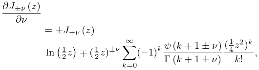
7: 10.15 Derivatives with Respect to Order

… ►

10.15.1 $$\frac{\partial J_{\pm \nu }\left(z\right)}{\partial \nu }=\pm J_{\pm \nu }\left(z\right)\ln \left(\frac{1}{2}z\right)\mp {(\frac{1}{2}z)}^{\pm \nu }\sum _{k=0}^{\mathrm{\infty }}{(-1)}^k\frac{\psi \left(k+1\pm \nu \right)}{\mathrm{\Gamma }\left(k+1\pm \nu \right)}\frac{{(\frac{1}{4}{z}^2)}^k}{k!},$$

ⓘ

Symbols:

$J_{\nu }\left(z\right)$: Bessel function of the first kind, $\mathrm{\Gamma }\left(z\right)$: gamma function, $\psi \left(z\right)$: psi (or digamma) function, $!$: factorial (as in $n!$), $\ln z$: principal branch of logarithm function, $\frac{\partial f}{\partial x}$: partial derivative of $f$ with respect to $x$ , $\partial x$: partial differential of $x$ , $k$: nonnegative integer, $z$: complex variable and $\nu$: complex parameter

A&S Ref:

9.1.64

Referenced by:

§10.15, §10.38, Erratum (V1.0.17) for Equations (10.15.1), (10.38.1)

Permalink:

http://dlmf.nist.gov/10.15.E1

Encodings:

pMML, png, TeX

Addition (effective with 1.0.17):

This equation has been generalized to include the additional case of $\partial J_{-\nu }\left(z\right)/\partial \nu$ because it will help the user who wants to combine it with (10.15.2).

See also:

Annotations for §10.15, §10.15 and Ch.10

…

8: 11.10 Anger–Weber Functions

… ►The Anger and Weber functions satisfy the inhomogeneous Bessel differential equation …

9: 2.8 Differential Equations with a Parameter

… ►For error bounds, extensions to pure imaginary or complex $u$, an extension to inhomogeneous differential equations, and examples, see Olver (1997b, Chapter 10). … ►For error bounds, more delicate error estimates, extensions to complex $\xi$ and $u$, zeros, connection formulas, extensions to inhomogeneous equations, and examples, see Olver (1997b, Chapters 11, 13), Olver (1964b), Reid (1974a, b), Boyd (1987), and Baldwin (1991). …

10: 14.29 Generalizations

… ►For inhomogeneous versions of the associated Legendre equation, and properties of their solutions, see Babister (1967, pp. 252–264).