DLMF: Untitled Document

… ►

See accompanying text — Figure 30.7.1: Eigenvalues $\lambda^{0}_{n}\left(\gamma^{2}\right)$ , $n=0,1,2,3$ , $-10\leq\gamma^{2}\leq 10$ . Magnify

►

… ►

…

… ►When any one of

j_{1},j_{2},j_{3}

is equal to

0,\tfrac{1}{2}

, or

1

, the

\mathit{3j}

symbol has a simple algebraic form. …For these and other results, and also cases in which any one of

j_{1},j_{2},j_{3}

is

\frac{3}{2}

or

2

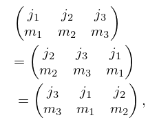
, see Edmonds (1974, pp. 125–127). … ►Even permutations of columns of a

\mathit{3j}

symbol leave it unchanged; odd permutations of columns produce a phase factor

(-1)^{j_{1}+j_{2}+j_{3}}

, for example, ►

34.3.8

\begin{pmatrix}j_{1}&j_{2}&j_{3}\\ m_{1}&m_{2}&m_{3}\end{pmatrix}=\begin{pmatrix}j_{2}&j_{3}&j_{1}\\ m_{2}&m_{3}&m_{1}\end{pmatrix}=\begin{pmatrix}j_{3}&j_{1}&j_{2}\\ m_{3}&m_{1}&m_{2}\end{pmatrix},

ⓘ

Symbols:: $\begin{pmatrix}\NVar{j_{1}}&\NVar{j_{2}}&\NVar{j_{3}}\\ \NVar{m_{1}}&\NVar{m_{2}}&\NVar{m_{3}}\end{pmatrix}$ : $\mathit{3j}$ symbol and $j,j_{r}$ : non-negative integers or non-negative integers plus one half.
Referenced by:: §34.3(ii)
Permalink:: http://dlmf.nist.gov/34.3.E8
Encodings:: pMML, png, TeX
See also:: Annotations for §34.3(ii), §34.3 and Ch.34

… ►For the polynomials

P_{l}

see §18.3, and for the function

Y_{{l},{m}}

see §14.30. …

… ►

\begin{pmatrix}j_{1}&j_{2}&j_{3}\\ m_{1}&m_{2}&m_{3}\end{pmatrix},

►

\begin{Bmatrix}j_{1}&j_{2}&j_{3}\\ l_{1}&l_{2}&l_{3}\end{Bmatrix},

►

\begin{Bmatrix}j_{11}&j_{12}&j_{13}\\ j_{21}&j_{22}&j_{23}\\ j_{31}&j_{32}&j_{33}\end{Bmatrix}.

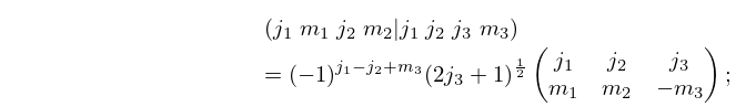
►An often used alternative to the

\mathit{3j}

symbol is the Clebsch–Gordan coefficient ►

34.1.1

\left(j_{1}\;m_{1}\;j_{2}\;m_{2}|j_{1}\;j_{2}\;j_{3}\,\,m_{3}\right)=(-1)^{j_{% 1}-j_{2}+m_{3}}(2j_{3}+1)^{\frac{1}{2}}\begin{pmatrix}j_{1}&j_{2}&j_{3}\\ m_{1}&m_{2}&-m_{3}\end{pmatrix};

ⓘ

Symbols:: $\begin{pmatrix}\NVar{j_{1}}&\NVar{j_{2}}&\NVar{j_{3}}\\ \NVar{m_{1}}&\NVar{m_{2}}&\NVar{m_{3}}\end{pmatrix}$ : $\mathit{3j}$ symbol and $j,j_{r}$ : non-negative integers or non-negative integers plus one half.
Sources:: Edmonds (1974, p. 46, Eq. (3.7.3)); Rotenberg et al. (1959, p. 1, Eq. (1.1a))
Permalink:: http://dlmf.nist.gov/34.1.E1
Encodings:: pMML, png, TeX
Clarification (effective with 1.0.15):: A wording change reflects that the Clebsch–Gordan coefficients are an alternative formulation of angular momentum problems, rather than alternative notation for the $\mathit{3j}$ . The sign of $m_{3}$ was changed for clarity.
See also:: Annotations for §34.1 and Ch.34

…

… ►

•

Abramowitz and Stegun (1964, Chapter 8) tabulates $\mathsf{P}_{n}\left(x\right)$ for $n=0(1)3,9,10$ , $x=0(.01)1$ , 5–8D; $\mathsf{P}_{n}'\left(x\right)$ for $n=1(1)4,9,10$ , $x=0(.01)1$ , 5–7D; $\mathsf{Q}_{n}\left(x\right)$ and $\mathsf{Q}_{n}'\left(x\right)$ for $n=0(1)3,9,10$ , $x=0(.01)1$ , 6–8D; $P_{n}\left(x\right)$ and $P_{n}'\left(x\right)$ for $n=0(1)5,9,10$ , $x=1(.2)10$ , 6S; $Q_{n}\left(x\right)$ and $Q_{n}'\left(x\right)$ for $n=0(1)3,9,10$ , $x=1(.2)10$ , 6S. (Here primes denote derivatives with respect to $x$ .)

►

•

Zhang and Jin (1996, Chapter 4) tabulates $\mathsf{P}_{n}\left(x\right)$ for $n=2(1)5,10$ , $x=0(.1)1$ , 7D; $\mathsf{P}_{n}\left(\cos\theta\right)$ for $n=1(1)4,10$ , $\theta=0(5^{\circ})90^{\circ}$ , 8D; $\mathsf{Q}_{n}\left(x\right)$ for $n=0(1)2,10$ , $x=0(.1)0.9$ , 8S; $\mathsf{Q}_{n}\left(\cos\theta\right)$ for $n=0(1)3,10$ , $\theta=0(5^{\circ})90^{\circ}$ , 8D; $\mathsf{P}^{m}_{n}\left(x\right)$ for $m=1(1)4$ , $n-m=0(1)2$ , $n=10$ , $x=0,0.5$ , 8S; $\mathsf{Q}^{m}_{n}\left(x\right)$ for $m=1(1)4$ , $n=0(1)2,10$ , 8S; $\mathsf{P}^{m}_{\nu}\left(\cos\theta\right)$ for $m=0(1)3$ , $\nu=0(.25)5$ , $\theta=0(15^{\circ})90^{\circ}$ , 5D; $P_{n}\left(x\right)$ for $n=2(1)5,10$ , $x=1(1)10$ , 7S; $Q_{n}\left(x\right)$ for $n=0(1)2,10$ , $x=2(1)10$ , 8S. Corresponding values of the derivative of each function are also included, as are 6D values of the first 5 $\nu$ -zeros of $\mathsf{P}^{m}_{\nu}\left(\cos\theta\right)$ and of its derivative for $m=0(1)4$ , $\theta=10^{\circ},30^{\circ},150^{\circ}$ .

►

•

Belousov (1962) tabulates $\mathsf{P}^{m}_{n}\left(\cos\theta\right)$ (normalized) for $m=0(1)36$ , $n-m=0(1)56$ , $\theta=0(2.5^{\circ})90^{\circ}$ , 6D.

►

•

Žurina and Karmazina (1964, 1965) tabulate the conical functions $\mathsf{P}_{-\frac{1}{2}+\mathrm{i}\tau}\left(x\right)$ for $\tau=0(.01)50$ , $x=-0.9(.1)0.9$ , 7S; $P_{-\frac{1}{2}+\mathrm{i}\tau}\left(x\right)$ for $\tau=0(.01)50$ , $x=1.1(.1)2(.2)5(.5)10(10)60$ , 7D. Auxiliary tables are included to facilitate computation for larger values of $\tau$ when $-1<x<1$ .

►

•

Žurina and Karmazina (1963) tabulates the conical functions $\mathsf{P}^{1}_{-\frac{1}{2}+\mathrm{i}\tau}\left(x\right)$ for $\tau=0(.01)25$ , $x=-0.9(.1)0.9$ , 7S; $P^{1}_{-\frac{1}{2}+\mathrm{i}\tau}\left(x\right)$ for $\tau=0(.01)25$ , $x=1.1(.1)2(.2)5(.5)10(10)60$ , 7S. Auxiliary tables are included to assist computation for larger values of $\tau$ when $-1<x<1$ .

…

… ►There is a unique point

z_{0}\in[\omega_{1},\omega_{1}+\omega_{3}]\cup[\omega_{1}+\omega_{3},\omega_{3}]

such that

\wp\left(z_{0}\right)=0

. … ►The interior of the rectangle with vertices

0

,

\omega_{1}

,

2\omega_{3}

,

2\omega_{3}-\omega_{1}

is mapped two-to-one onto the lower half-plane. The interior of the rectangle with vertices

0

,

\omega_{1}

,

\frac{1}{2}\omega_{1}+\omega_{3}

,

\frac{1}{2}\omega_{1}-\omega_{3}

is mapped one-to-one onto the lower half-plane with a cut from

e_{3}

to

\wp\left(\frac{1}{2}\omega_{1}+\omega_{3}\right)\>(=\wp\left(\frac{1}{2}\omega% _{1}-\omega_{3}\right))

. The cut is the image of the edge from

\frac{1}{2}\omega_{1}+\omega_{3}

to

\frac{1}{2}\omega_{1}-\omega_{3}

and is not a line segment. … ►The order of a point (if finite and not already determined) can have only the values 3, 5, 6, 7, 9, 10, or 12, and so can be found from

2P=-P

,

4P=-P

,

4P=-2P

,

8P=P

,

8P=-P

,

8P=-2P

, or

8P=-4P

. …

… ►Let …where … ►Next, for

j=1,2

, define

Q_{j}(t)=f_{j}+g_{j}t+h_{j}t^{2}

, and assume both

Q

’s are positive for

y<t<x

. …where …If

Q_{1}(t)=(a_{1}+b_{1}t)(a_{2}+b_{2}t)

, where both linear factors are positive for

y<t<x

, and

Q_{2}(t)=f_{2}+g_{2}t+h_{2}t^{2}

, then (19.29.25) is modified so that …

… ►

•

Achenbach (1986) tabulates $J_{0}\left(x\right)$ , $J_{1}\left(x\right)$ , $Y_{0}\left(x\right)$ , $Y_{1}\left(x\right)$ , $x=0(.1)8$ , 20D or 18–20S.

… ►

•

Kerimov and Skorokhodov (1985c) tabulates 201 double zeros of $J_{-\nu}''\left(x\right)$ , 10 double zeros of $J_{-\nu}'''\left(x\right)$ , 101 double zeros of $Y_{-\nu}'\left(x\right)$ , 201 double zeros of $Y_{-\nu}''\left(x\right)$ , and 10 double zeros of $Y_{-\nu}'''\left(x\right)$ , all to 8 or 9D.

… ►

•

Achenbach (1986) tabulates $I_{0}\left(x\right)$ , $I_{1}\left(x\right)$ , $K_{0}\left(x\right)$ , $K_{1}\left(x\right)$ , $x=0(.1)8$ , 19D or 19–21S.

… ►

•

The main tables in Abramowitz and Stegun (1964, Chapter 10) give $\mathsf{j}_{n}\left(x\right)$ , $\mathsf{y}_{n}\left(x\right)$ $n=0(1)8$ , $x=0(.1)10$ , 5–8S; $\mathsf{j}_{n}\left(x\right)$ , $\mathsf{y}_{n}\left(x\right)$ $n=0(1)20(10)50$ , 100, $x=1,2,5,10,50,100$ , 10S; ${\mathsf{i}^{(1)}_{n}}\left(x\right)$ , $\mathsf{k}_{n}\left(x\right)$ , $n=0,1,2$ , $x=0(.1)5$ , 4–9D; ${\mathsf{i}^{(1)}_{n}}\left(x\right)$ , $\mathsf{k}_{n}\left(x\right)$ , $n=0(1)20(10)50$ , 100, $x=1,2,5,10,50,100$ , 10S. (For the notation see §10.1 and §10.47(ii).)

… ►

•

Young and Kirk (1964) tabulates $\operatorname{ber}_{n}x$ , $\operatorname{bei}_{n}x$ , $\operatorname{ker}_{n}x$ , $\operatorname{kei}_{n}x$ , $n=0,1$ , $x=0(.1)10$ , 15D; $\operatorname{ber}_{n}x$ , $\operatorname{bei}_{n}x$ , $\operatorname{ker}_{n}x$ , $\operatorname{kei}_{n}x$ , modulus and phase functions $M_{n}\left(x\right)$ , $\theta_{n}\left(x\right)$ , $N_{n}\left(x\right)$ , $\phi_{n}\left(x\right)$ , $n=0,1,2$ , $x=0(.01)2.5$ , 8S, and $n=0(1)10$ , $x=0(.1)10$ , 7S. Also included are auxiliary functions to facilitate interpolation of the tables for $n=0(1)10$ for small values of $x$ . (Concerning the phase functions see §10.68(iv).)

…

… ►where

u_{j}=c_{j}

,

j=1,2,\dots,n-1

,

d_{1}=b_{1}

, and …Forward elimination for solving

\mathbf{A}\mathbf{x}=\mathbf{f}

then becomes

y_{1}=f_{1}

, …and back substitution is

x_{n}=y_{n}/d_{n}

, followed by … ►Define the Lanczos vectors

\mathbf{v}_{j}

and coefficients

\alpha_{j}

and

\beta_{j}

by

\mathbf{v}_{0}=\boldsymbol{{0}}

, a normalized vector

\mathbf{v}_{1}

(perhaps chosen randomly),

\alpha_{1}=\mathbf{v}_{1}^{\rm T}\mathbf{A}\mathbf{v}_{1}

,

\beta_{1}=0

, and for

j=1,2,\ldots,n-1

by the recursive scheme … ►Start with

\mathbf{v}_{0}=\boldsymbol{{0}}

, vector

\mathbf{v}_{1}

such that

\mathbf{v}_{1}^{\rm T}\mathbf{S}\mathbf{v}_{1}=1

,

\alpha_{1}=\mathbf{v}_{1}^{\rm T}\mathbf{A}\mathbf{v}_{1}

,

\beta_{1}=0

. …

… ►where

w_{1}

and

w_{2}

are any solutions of (9.2.1). … ►where

J_{0}

is the Bessel function (§10.2(ii)). … ►Let

w_{1},w_{2}

be any solutions of (9.2.1), not necessarily distinct. … ►

9.11.10

\int zw^{\prime}_{1}w^{\prime}_{2}\,\mathrm{d}z=\tfrac{3}{10}(-w_{1}w_{2}+zw_{% 1}w^{\prime}_{2}+zw^{\prime}_{1}w_{2})+\tfrac{1}{5}(z^{2}w^{\prime}_{1}w^{% \prime}_{2}-z^{3}w_{1}w_{2}).

ⓘ

Symbols:: $\,\mathrm{d}\NVar{x}$ : differential of $x$ , $\int$ : integral, $z$ : complex variable and $w$ : function
Source:: Albright (1977, (A.21))
Permalink:: http://dlmf.nist.gov/9.11.E10
Encodings:: pMML, png, TeX
See also:: Annotations for §9.11(iv), §9.11 and Ch.9

►For

\int z^{n}w_{1}w_{2}\,\mathrm{d}z

,

\int z^{n}w_{1}w^{\prime}_{2}\,\mathrm{d}z

,

\int z^{n}w^{\prime}_{1}w^{\prime}_{2}\,\mathrm{d}z

, where

n

is any positive integer, see Albright (1977). …

… ►For a given integer

k\geq 2

the function

r_{k}\left(n\right)

is defined as the number of solutions of the equation …where the

x_{j}

are integers, positive, negative, or zero, and the order of the summands is taken into account. … ►Hence

r_{2}\left(5\right)=8

because both divisors,

1

and

5

, are congruent to

1\pmod{4}

. … ►By similar methods Jacobi proved that

r_{4}\left(n\right)=8\sigma_{1}\left(n\right)

if

n

is odd, whereas, if

n

is even,

r_{4}\left(n\right)=24

times the sum of the odd divisors of

n

. …Explicit formulas for

r_{k}\left(n\right)

have been obtained by similar methods for

k=6,8,10

, and

12

, but they are more complicated. …

.2022世界杯中国男足蠃_『wn4.com_』世界杯冠军加多少分_w2n3c1o_2022年12月10日16时49分8秒_zwuzf2w8s

21—30 of 815 matching pages

21: 30.7 Graphics

22: 34.3 Basic Properties: $\mathit{3j}$ Symbol

23: 34.1 Special Notation

24: 14.33 Tables

25: 23.20 Mathematical Applications

26: 19.29 Reduction of General Elliptic Integrals

27: 10.75 Tables

28: 3.2 Linear Algebra

29: 9.11 Products

30: 27.13 Functions