.竞彩可以买单场吗『网址:mxsty.cc』.进世界杯的要求.m6q3s2-2022年12月10日16时2分3秒

Did you mean .竞彩可以买单场吗『网址:style』.进世界杯的要求.m6q3s2-2022年12月10日16时2分3秒 ?

(0.006 seconds)

1—10 of 611 matching pages

1: 34.2 Definition: $\mathit{3j}$ Symbol

§34.2 Definition: $\mathit{3j}$ Symbol

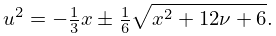
►The quantities

j_{1},j_{2},j_{3}

in the

\mathit{3j}

symbol are called angular momenta. …They therefore satisfy the triangle conditions …where

r, s, t

is any permutation of

1,2,3

. The corresponding projective quantum numbers

m_{1},m_{2},m_{3}

are given by …

2: 11 Struve and Related Functions

…

3: 8.26 Tables

… ►

•

Zhang and Jin (1996, Table 3.8) tabulates $\gamma\left(a,x\right)$ for $a=0.5,1,3,5,10,25,50,100$ , $x=0(.1)1(1)3,5(5)30,50,100$ to 8D or 8S.

… ►

•

Zhang and Jin (1996, Table 3.9) tabulates $I_{x}\left(a,b\right)$ for $x=0(.05)1$ , $a=0.5,1,3,5,10$ , $b=1,10$ to 8D.

… ►

•

Abramowitz and Stegun (1964, pp. 245–248) tabulates $E_{n}\left(x\right)$ for $n=2,3,4,10,20$ , $x=0(.01)2$ to 7D; also $(x+n)e^{x}E_{n}\left(x\right)$ for $n=2,3,4,10,20$ , $x^{-1}=0(.01)0.1(.05)0.5$ to 6S.

… ►

•

Pagurova (1961) tabulates $E_{n}\left(x\right)$ for $n=0(1)20$ , $x=0(.01)2(.1)10$ to 4-9S; $e^{x}E_{n}\left(x\right)$ for $n=2(1)10$ , $x=10(.1)20$ to 7D; $e^{x}E_{p}\left(x\right)$ for $p=0(.1)1$ , $x=0.01(.01)7(.05)12(.1)20$ to 7S or 7D.

… ►

•

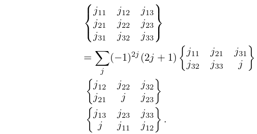
Zhang and Jin (1996, Table 19.1) tabulates $E_{n}\left(x\right)$ for $n=1,2,3,5,10,15,20$ , $x=0(.1)1,1.5,2,3,5,10,20,30,50,100$ to 7D or 8S.

4: 34.11 Higher-Order $3nj$ Symbols

§34.11 Higher-Order $3nj$ Symbols

►For information on

12j,15j

,…, symbols, see Varshalovich et al. (1988, §10.12) and Yutsis et al. (1962, pp. 62–65 and 122–153).

5: 32.3 Graphics

… ►

See accompanying text — Figure 32.3.3: $w_{k}(x)$ for $-12\leq x\leq 0.73$ and $k=1.85185\;3$ , $1.85185\;5$ . … Magnify

►

… ►

32.3.6

u^{2}=-\tfrac{1}{3}x\pm\tfrac{1}{6}\sqrt{x^{2}+12\nu+6}.

ⓘ

Symbols:: $x$ : real, $\nu$ : parameter and $u_{k}(x;\nu)$ : solution
Permalink:: http://dlmf.nist.gov/32.3.E6
Encodings:: pMML, png, TeX
See also:: Annotations for §32.3(iii), §32.3 and Ch.32

… ►

►

…

6: 18.41 Tables

… ►Abramowitz and Stegun (1964, Tables 22.4, 22.6, 22.11, and 22.13) tabulates

T_{n}\left(x\right)

U_{n}\left(x\right)

L_{n}\left(x\right)

, and

H_{n}\left(x\right)

for

n=0(1)12

. The ranges of

x

are

0.2(.2)1

for

T_{n}\left(x\right)

and

U_{n}\left(x\right)

, and

0.5,1,3,5,10

for

L_{n}\left(x\right)

and

H_{n}\left(x\right)

. …

7: 34.6 Definition: $\mathit{9j}$ Symbol

… ►The

\mathit{9j}

symbol may be defined either in terms of

\mathit{3j}

symbols or equivalently in terms of

\mathit{6j}

symbols: ►

34.6.1

\begin{Bmatrix}j_{11}&j_{12}&j_{13}\\ j_{21}&j_{22}&j_{23}\\ j_{31}&j_{32}&j_{33}\end{Bmatrix}=\sum_{\mbox{\scriptsize all }m_{rs}}\begin{% pmatrix}j_{11}&j_{12}&j_{13}\\ m_{11}&m_{12}&m_{13}\end{pmatrix}\begin{pmatrix}j_{21}&j_{22}&j_{23}\\ m_{21}&m_{22}&m_{23}\end{pmatrix}\begin{pmatrix}j_{31}&j_{32}&j_{33}\\ m_{31}&m_{32}&m_{33}\end{pmatrix}\*\begin{pmatrix}j_{11}&j_{21}&j_{31}\\ m_{11}&m_{21}&m_{31}\end{pmatrix}\begin{pmatrix}j_{12}&j_{22}&j_{32}\\ m_{12}&m_{22}&m_{32}\end{pmatrix}\begin{pmatrix}j_{13}&j_{23}&j_{33}\\ m_{13}&m_{23}&m_{33}\end{pmatrix},

ⓘ

Defines:: $\begin{Bmatrix}\NVar{j_{11}}&\NVar{j_{12}}&\NVar{j_{13}}\\ \NVar{j_{21}}&\NVar{j_{22}}&\NVar{j_{23}}\\ \NVar{j_{31}}&\NVar{j_{32}}&\NVar{j_{33}}\end{Bmatrix}$ : $\mathit{9j}$ symbol
Symbols:: $\begin{pmatrix}\NVar{j_{1}}&\NVar{j_{2}}&\NVar{j_{3}}\\ \NVar{m_{1}}&\NVar{m_{2}}&\NVar{m_{3}}\end{pmatrix}$ : $\mathit{3j}$ symbol, $j,j_{r}$ : non-negative integers or non-negative integers plus one half., $r$ : nonnegative integer and $s$ : integer
Permalink:: http://dlmf.nist.gov/34.6.E1
Encodings:: pMML, png, TeX
See also:: Annotations for §34.6 and Ch.34

►

34.6.2

\begin{Bmatrix}j_{11}&j_{12}&j_{13}\\ j_{21}&j_{22}&j_{23}\\ j_{31}&j_{32}&j_{33}\end{Bmatrix}=\sum_{j}(-1)^{2j}(2j+1)\begin{Bmatrix}j_{11}% &j_{21}&j_{31}\\ j_{32}&j_{33}&j\end{Bmatrix}\begin{Bmatrix}j_{12}&j_{22}&j_{32}\\ j_{21}&j&j_{23}\end{Bmatrix}\begin{Bmatrix}j_{13}&j_{23}&j_{33}\\ j&j_{11}&j_{12}\end{Bmatrix}.

ⓘ

Symbols:: $\begin{Bmatrix}\NVar{j_{11}}&\NVar{j_{12}}&\NVar{j_{13}}\\ \NVar{j_{21}}&\NVar{j_{22}}&\NVar{j_{23}}\\ \NVar{j_{31}}&\NVar{j_{32}}&\NVar{j_{33}}\end{Bmatrix}$ : $\mathit{9j}$ symbol, $\begin{Bmatrix}\NVar{j_{1}}&\NVar{j_{2}}&\NVar{j_{3}}\\ \NVar{l_{1}}&\NVar{l_{2}}&\NVar{l_{3}}\end{Bmatrix}$ : $\mathit{6j}$ symbol and $j,j_{r}$ : non-negative integers or non-negative integers plus one half.
Referenced by:: §34.13
Permalink:: http://dlmf.nist.gov/34.6.E2
Encodings:: pMML, png, TeX
See also:: Annotations for §34.6 and Ch.34

…

8: 25.20 Approximations

… ►

•

Piessens and Branders (1972) gives the coefficients of the Chebyshev-series expansions of $s\zeta\left(s+1\right)$ and $\zeta\left(s+k\right)$ , $k=2,3,4,5,8$ , for $0\leq s\leq 1$ (23D).

… ►

•

Antia (1993) gives minimax rational approximations for $\Gamma\left(s+1\right)F_{s}(x)$ , where $F_{s}(x)$ is the Fermi–Dirac integral (25.12.14), for the intervals $-\infty<x\leq 2$ and $2\leq x<\infty$ , with $s=-\frac{1}{2},\frac{1}{2},\frac{3}{2},\frac{5}{2}$ . For each $s$ there are three sets of approximations, with relative maximum errors $10^{-4},10^{-8},10^{-12}$ .

9: Staff

… ►

Leonard C. Maximon, George Washington University, Chaps. 10, 34

… ►

Frank W. J. Olver, University of Maryland and NIST, Chaps. 1, 2, 4, 9, 10

… ►

Nico M. Temme, Centrum Wiskunde Informatica, Chaps. 3, 6, 7, 12

… ►

Diego Dominici, State University of New York at New Paltz, for Chaps. 9, 10 (deceased)

… ►

Nico M. Temme, Centrum Wiskunde & Informatica (CWI), for Chaps. 3, 6, 7, 12

…

10: 11.14 Tables

… ►

•

Abramowitz and Stegun (1964, Chapter 12) tabulates $\mathbf{H}_{n}\left(x\right)$ , $\mathbf{H}_{n}\left(x\right)-Y_{n}\left(x\right)$ , and $I_{n}\left(x\right)-\mathbf{L}_{n}\left(x\right)$ for $n=0,1$ and $x=0(.1)5$ , $x^{-1}=0(.01)0.2$ to 6D or 7D.

… ►

•

Barrett (1964) tabulates $\mathbf{L}_{n}\left(x\right)$ for $n=0,1$ and $x=0.2(.005)4(.05)10(.1)19.2$ to 5 or 6S, $x=6(.25)59.5(.5)100$ to 2S.

… ►

•

Abramowitz and Stegun (1964, Chapter 12) tabulates $\int_{0}^{x}(I_{0}\left(t\right)-\mathbf{L}_{0}\left(t\right))\,\mathrm{d}t$ and $(2/\pi)\int_{x}^{\infty}t^{-1}\mathbf{H}_{0}\left(t\right)\,\mathrm{d}t$ for $x=0(.1)5$ to 5D or 7D; $\int_{0}^{x}(\mathbf{H}_{0}\left(t\right)-Y_{0}\left(t\right))\,\mathrm{d}t-(2% /\pi)\ln x$ , $\int_{0}^{x}(I_{0}\left(t\right)-\mathbf{L}_{0}\left(t\right))\,\mathrm{d}t-(2% /\pi)\ln x$ , and $\int_{x}^{\infty}t^{-1}(\mathbf{H}_{0}\left(t\right)-Y_{0}\left(t\right))\,% \mathrm{d}t$ for $x^{-1}=0(.01)0.2$ to 6D.

… ►

•

Bernard and Ishimaru (1962) tabulates $\mathbf{J}_{\nu}\left(x\right)$ and $\mathbf{E}_{\nu}\left(x\right)$ for $\nu=-10(.1)10$ and $x=0(.1)10$ to 5D.

… ►

•

Agrest and Maksimov (1971, Chapter 11) defines incomplete Struve, Anger, and Weber functions and includes tables of an incomplete Struve function $\mathbf{H}_{n}\left(x,\alpha\right)$ for $n=0,1$ , $x=0(.2)10$ , and $\alpha=0(.2)1.4,\tfrac{1}{2}\pi$ , together with surface plots.