with respect to order

SearchAdvancedHelp

(0.008 seconds)

31—40 of 136 matching pages

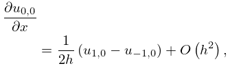
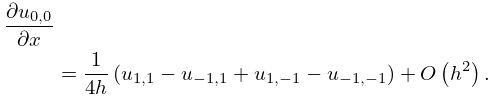
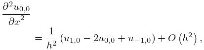
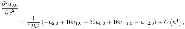
31: 3.4 Differentiation

… ►

3.4.20 $$\frac{\partial u_{0,0}}{\partial x}=\frac{1}{2h}(u_{1,0}-u_{-1,0})+O\left(h^2\right),$$

ⓘ

Symbols:

$O\left(x\right)$: order not exceeding, $\frac{\partial f}{\partial x}$: partial derivative of $f$ with respect to $x$ , $\partial x$: partial differential of $x$ and $u$: function

A&S Ref:

25.3.21

Permalink:

http://dlmf.nist.gov/3.4.E20

Encodings:

pMML, png, TeX

See also:

Annotations for §3.4(iii), §3.4(iii), §3.4 and Ch.3

►

3.4.21 $$\frac{\partial u_{0,0}}{\partial x}=\frac{1}{4h}(u_{1,1}-u_{-1,1}+u_{1,-1}-u_{-1,-1})+O\left(h^2\right).$$

ⓘ

Symbols:

$O\left(x\right)$: order not exceeding, $\frac{\partial f}{\partial x}$: partial derivative of $f$ with respect to $x$ , $\partial x$: partial differential of $x$ and $u$: function

A&S Ref:

25.3.22

Permalink:

http://dlmf.nist.gov/3.4.E21

Encodings:

pMML, png, TeX

See also:

Annotations for §3.4(iii), §3.4(iii), §3.4 and Ch.3

… ►

3.4.22 $$\frac{{\partial }^2{u}_{0,0}}{{\partial x}^2}=\frac{1}{h^2}(u_{1,0}-2u_{0,0}+u_{-1,0})+O\left(h^2\right),$$

ⓘ

Symbols:

$O\left(x\right)$: order not exceeding, $\frac{\partial f}{\partial x}$: partial derivative of $f$ with respect to $x$ , $\partial x$: partial differential of $x$ and $u$: function

A&S Ref:

25.3.23

Permalink:

http://dlmf.nist.gov/3.4.E22

Encodings:

pMML, png, TeX

See also:

Annotations for §3.4(iii), §3.4(iii), §3.4 and Ch.3

►

3.4.23 $$\frac{{\partial }^2{u}_{0,0}}{{\partial x}^2}=\frac{1}{12h^2}(-u_{2,0}+16u_{1,0}-30u_{0,0}+16u_{-1,0}-u_{-2,0})+O\left(h^4\right),$$

ⓘ

Symbols:

$O\left(x\right)$: order not exceeding, $\frac{\partial f}{\partial x}$: partial derivative of $f$ with respect to $x$ , $\partial x$: partial differential of $x$ and $u$: function

A&S Ref:

25.3.24

Permalink:

http://dlmf.nist.gov/3.4.E23

Encodings:

pMML, png, TeX

See also:

Annotations for §3.4(iii), §3.4(iii), §3.4 and Ch.3

►

3.4.24 $$\frac{{\partial }^2{u}_{0,0}}{{\partial x}^2}=\frac{1}{3h^2}(u_{1,1}-2u_{0,1}+u_{-1,1}+u_{1,0}-2u_{0,0}+u_{-1,0}+u_{1,-1}-2u_{0,-1}+u_{-1,-1})+O\left(h^2\right).$$

ⓘ

Symbols:

$O\left(x\right)$: order not exceeding, $\frac{\partial f}{\partial x}$: partial derivative of $f$ with respect to $x$ , $\partial x$: partial differential of $x$ and $u$: function

A&S Ref:

25.3.25

Permalink:

http://dlmf.nist.gov/3.4.E24

Encodings:

pMML, png, TeX

See also:

Annotations for §3.4(iii), §3.4(iii), §3.4 and Ch.3

…

32: 11.10 Anger–Weber Functions

… ►

11.10.5 $$\frac{d^{2}w}{{dz}^2}+\frac{1}{z}\frac{dw}{dz}+\left(1-\frac{{\nu }^2}{z^2}\right)w=f(\nu ,z),$$

ⓘ

Symbols:

$\frac{df}{dx}$: derivative of $f$ with respect to $x$ , $z$: complex variable and $\nu$: real or complex order

Permalink:

http://dlmf.nist.gov/11.10.E5

Encodings:

pMML, png, TeX

See also:

Annotations for §11.10(ii), §11.10 and Ch.11

… ►

11.10.27 $${\frac{\partial }{\partial \nu }{𝐉}_{\nu }\left(z\right)|}_{\nu =0}=\frac{1}{2}\pi {𝐇}_0\left(z\right),$$

ⓘ

Symbols:

${𝐉}_{\nu }\left(z\right)$: Anger function, ${𝐇}_{\nu }\left(z\right)$: Struve function, $\pi$: the ratio of the circumference of a circle to its diameter, $\frac{\partial f}{\partial x}$: partial derivative of $f$ with respect to $x$ , $\partial x$: partial differential of $x$ , $z$: complex variable and $\nu$: real or complex order

Referenced by:

§11.10(vii)

Permalink:

http://dlmf.nist.gov/11.10.E27

Encodings:

pMML, png, TeX

See also:

Annotations for §11.10(vii), §11.10 and Ch.11

►

11.10.28 $${\frac{\partial }{\partial \nu }{𝐄}_{\nu }\left(z\right)|}_{\nu =0}=\frac{1}{2}\pi J_0\left(z\right).$$

ⓘ

Symbols:

$J_{\nu }\left(z\right)$: Bessel function of the first kind, ${𝐄}_{\nu }\left(z\right)$: Weber function, $\pi$: the ratio of the circumference of a circle to its diameter, $\frac{\partial f}{\partial x}$: partial derivative of $f$ with respect to $x$ , $\partial x$: partial differential of $x$ , $z$: complex variable and $\nu$: real or complex order

Referenced by:

§11.10(vii)

Permalink:

http://dlmf.nist.gov/11.10.E28

Encodings:

pMML, png, TeX

See also:

Annotations for §11.10(vii), §11.10 and Ch.11

…

33: 14.15 Uniform Asymptotic Approximations

… ►as $\mu \to \mathrm{\infty }$, uniformly with respect to $x$. … ►For the interval the following asymptotic approximations hold when $\mu \to \mathrm{\infty }$, with $\nu$ ($\ge -\frac{1}{2}$) fixed, uniformly with respect to $x$: … ►uniformly with respect to $x\in (1,\mathrm{\infty })$ and $\nu +\frac{1}{2}\in [0,(1-\delta )\mu ]$. …The interval is mapped one-to-one to the interval , with the points $x=1$ and $x=\mathrm{\infty }$ corresponding to $\eta =\mathrm{\infty }$ and $\eta =0$, respectively. … ►When $a=0$ the interval is mapped one-to-one to the interval , with the points $x=-1$, $0$, and $1$ corresponding to $\zeta =-\mathrm{\infty }$, $0$, and $\mathrm{\infty }$, respectively. …

34: 10.20 Uniform Asymptotic Expansions for Large Order

… ►For asymptotic properties of the expansions (10.20.4)–(10.20.6) with respect to large values of $z$ see §10.41(v).

35: 36.11 Leading-Order Asymptotics

… ►

36.11.2 $${\mathrm{\Psi }}_K\left(𝐱\right)=\sqrt{2\pi }\sum _{j=1}^{j_{\max }(𝐱)}\exp \left(\mathrm{i}\left({\mathrm{\Phi }}_K(t_j(𝐱);𝐱)+\frac{1}{4}\pi {(-1)}^{j+K+1}\right)\right){\left|\frac{{\partial }^2{\mathrm{\Phi }}_K(t_j(𝐱);𝐱)}{{\partial t}^2}\right|}^{-1/2}(1+o\left(1\right)).$$

ⓘ

Symbols:

${\mathrm{\Psi }}_K\left(𝐱\right)$: canonical integral function, $\pi$: the ratio of the circumference of a circle to its diameter, ${\mathrm{\Phi }}_K(t;𝐱)$: cuspoid catastrophe of codimension $K$ , $\exp z$: exponential function, $\mathrm{i}$: imaginary unit, $o\left(x\right)$: order less than, $\frac{\partial f}{\partial x}$: partial derivative of $f$ with respect to $x$ , $\partial x$: partial differential of $x$ , $t$: variable, $K$: codimension and $t_j(𝐱)$: solutions

Permalink:

http://dlmf.nist.gov/36.11.E2

Encodings:

pMML, png, TeX

See also:

Annotations for §36.11 and Ch.36

…

36: 28.12 Definitions and Basic Properties

… ►As in §28.7 values of $q$ for which (28.2.16) has simple roots $\lambda$ are called normal values with respect to $\nu$. … ►

§28.12(ii) Eigenfunctions ${\mathrm{me}}_{\nu }(z,q)$

… ►The Floquet solution with respect to $\nu$ is denoted by ${\mathrm{me}}_{\nu }(z,q)$. … ► … ►

37: 14.20 Conical (or Mehler) Functions

… ►

14.20.1 $$\left(1-x^2\right)\frac{d^{2}w}{{dx}^2}-2x\frac{dw}{dx}-\left({\tau }^2+\frac{1}{4}+\frac{{\mu }^2}{1-x^2}\right)w=0.$$

ⓘ

Symbols:

$\frac{df}{dx}$: derivative of $f$ with respect to $x$ , $x$: real variable, $\tau$: real variable and $\mu$: general order

Referenced by:

§14.20(i), §14.20(i), 2nd item

Permalink:

http://dlmf.nist.gov/14.20.E1

Encodings:

pMML, png, TeX

See also:

Annotations for §14.20(i), §14.20 and Ch.14

…

38: Mathematical Introduction

… ►In these cases the phase colors that correspond to the 1st, 2nd, 3rd, and 4th quadrants are arranged in alphabetical order: blue, green, red, and yellow, respectively, and a “Quadrant Colors” icon appears alongside the figure. …

39: 6.13 Zeros

… ► $\mathrm{Ci}\left(x\right)$ and $\mathrm{si}\left(x\right)$ each have an infinite number of positive real zeros, which are denoted by $c_k$, $s_k$, respectively, arranged in ascending order of absolute value for $k=0,1,2,\mathrm{\dots }$. Values of $c_1$ and $c_2$ to 30D are given by MacLeod (1996b). ►As $k\to \mathrm{\infty }$, …

40: 1.13 Differential Equations

… ►(More generally in (1.13.5) for $n$th-order differential equations, $f(z)$ is the coefficient multiplying the $(n-1)$th-order derivative of the solution divided by the coefficient multiplying the $n$th-order derivative of the solution, see Ince (1926, §5.2).) … ► $u$ and $z$ belong to domains $U$ and $D$ respectively, the coefficients $f(u,z)$ and $g(u,z)$ are continuous functions of both variables, and for each fixed $u$ (fixed $z$) the two functions are analytic in $z$ (in $u$). … ►Here dots denote differentiations with respect to $\zeta$, and $\{z,\zeta \}$ is the Schwarzian derivative: … ►For extensions of these results to linear homogeneous differential equations of arbitrary order see Spigler (1984). … ►For an extensive collection of solutions of differential equations of the first, second, and higher orders see Kamke (1977). …