with respect to integration
(0.006 seconds)
41—50 of 63 matching pages
41: 32.10 Special Function Solutions
…
►
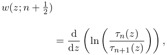
32.10.8
…
►When is zero or a negative integer the parabolic cylinder functions reduce to Hermite polynomials (§18.3) times an exponential function; thus
…
►
32.10.22
…
►
32.10.33
…
►The solution (32.10.34) is an essentially transcendental function of both constants of integration since with and does not admit an algebraic first integral of the form , with a constant.
…
42: 3.7 Ordinary Differential Equations
…
►Consideration will be limited to ordinary linear second-order
differential equations
…For applications to special functions , , and are often simple rational functions.
…
►Assume that we wish to integrate (3.7.1) along a finite path from
to
in a domain .
…
►The larger the absolute values of the eigenvalues that are being sought, the smaller the integration steps need to be.
…
►The Runge–Kutta method applies to linear or nonlinear differential equations.
…
43: 36.12 Uniform Approximation of Integrals
…
►In the cuspoid case (one integration variable)
…
►Define a mapping by relating
to the normal form (36.2.1) of in the following way:
…
►This technique can be applied to generate a hierarchy of approximations for the diffraction catastrophes in (36.2.10) away from , in terms of canonical integrals for .
For example, the diffraction catastrophe defined by (36.2.10), and corresponding to the Pearcey integral (36.2.14), can be approximated by the Airy function when is large, provided that and are not small.
…
►Also, and are chosen to be positive real when is such that both critical points are real, and by analytic continuation otherwise.
…
44: 2.10 Sums and Sequences
…
►Assume that , and are integers such that , , and is absolutely integrable over .
Then
…
►
(a)
…
►This identity can be used to find asymptotic approximations for large when the factor changes slowly with , and is oscillatory; compare the approximation of Fourier integrals by integration by parts in §2.3(i).
…
►In these circumstances the integrals in (2.10.28) are integrable by parts times, yielding
…
On the strip , is analytic in its interior, is continuous on its closure, and as , uniformly with respect to .
45: 1.6 Vectors and Vector-Valued Functions
…
►where is the unit vector normal to
and whose direction is determined by the right-hand rule; see Figure 1.6.1.
…
►If and , then the reparametrization is called orientation-preserving, and
…If and , then the reparametrization is orientation-reversing and
…
►are tangent to the surface at .
…
►If and are both orientation preserving or both orientation reversing parametrizations of defined on open sets and
respectively, then
…
46: 21.7 Riemann Surfaces
…
►Although there are other ways to represent Riemann surfaces (see e.
…To accomplish this we write (21.7.1) in terms of homogeneous coordinates:
…
►Note that for the purposes of integrating these holomorphic differentials, all cycles on the surface are a linear combination of the cycles , , .
…
►where and are points on , , and the path of integration on from
to
is identical for all components.
…
►where again all integration paths are identical for all components.
…
47: 10.43 Integrals
…
►
(a)
…
►For collections of integrals of the functions and , including integrals with respect to the order, see Apelblat (1983, §12), Erdélyi et al. (1953b, §§7.7.1–7.7.7 and 7.14–7.14.2), Erdélyi et al. (1954a, b), Gradshteyn and Ryzhik (2000, §§5.5, 6.5–6.7), Gröbner and Hofreiter (1950, pp. 197–203), Luke (1962), Magnus et al. (1966, §3.8), Marichev (1983, pp. 191–216), Oberhettinger (1972), Oberhettinger (1974, §§1.11 and 2.7), Oberhettinger (1990, §§1.17–1.20 and 2.17–2.20), Oberhettinger and Badii (1973, §§1.15 and 2.13), Okui (1974, 1975), Prudnikov et al. (1986b, §§1.11–1.12, 2.15–2.16, 3.2.8–3.2.10, and 3.4.1), Prudnikov et al. (1992a, §§3.15, 3.16), Prudnikov et al. (1992b, §§3.15, 3.16), Watson (1944, Chapter 13), and Wheelon (1968).
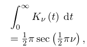
10.43.15
.
►
10.43.16
.
…
►
10.43.18
.
…
►
On the interval , is continuously differentiable and each of and is absolutely integrable.
48: 2.1 Definitions and Elementary Properties
…
►
§2.1(ii) Integration and Differentiation
►Integration of asymptotic and order relations is permissible, subject to obvious convergence conditions. … ►The asymptotic property may also hold uniformly with respect to parameters. …as in , uniformly with respect to . … ►As in §2.1(iv), generalized asymptotic expansions can also have uniformity properties with respect to parameters. …49: 9.13 Generalized Airy Functions
…
►are used in approximating solutions to differential equations with multiple turning points; see §2.8(v).
…
►When , and become and , respectively.
…
►As
…
►(The overbar has nothing to do with complex conjugates.)
…
►The integration paths , , , are depicted in Figure 9.13.1.
…
50: 10.22 Integrals
…
►In this subsection and denote cylinder functions(§10.2(ii)) of orders and , respectively, not necessarily distinct.
…
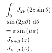
►
10.22.15
.
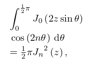
►
10.22.16
.
…
►For the Ferrers function and the associated Legendre function , see §§14.3(i) and 14.3(ii), respectively.
…
►For collections of integrals of the functions , , , and , including integrals with respect to the order, see Andrews et al. (1999, pp. 216–225), Apelblat (1983, §12), Erdélyi et al. (1953b, §§7.7.1–7.7.7 and 7.14–7.14.2), Erdélyi et al. (1954a, b), Gradshteyn and Ryzhik (2000, §§5.5 and 6.5–6.7), Gröbner and Hofreiter (1950, pp. 196–204), Luke (1962), Magnus et al. (1966, §3.8), Marichev (1983, pp. 191–216), Oberhettinger (1974, §§1.10 and 2.7), Oberhettinger (1990, §§1.13–1.16 and 2.13–2.16), Oberhettinger and Badii (1973, §§1.14 and 2.12), Okui (1974, 1975), Prudnikov et al. (1986b, §§1.8–1.10, 2.12–2.14,
3.2.4–3.2.7, 3.3.2, and 3.4.1), Prudnikov et al. (1992a, §§3.12–3.14), Prudnikov et al. (1992b, §§3.12–3.14), Watson (1944, Chapters 5, 12, 13, and 14), and Wheelon (1968).
