tangent numbers

SearchAdvancedHelp

(0.001 seconds)

11—20 of 24 matching pages

11: Guide to Searching the DLMF

… ►

Table 1: Query Examples

► ►►►

Query	Matching records contain
…
trigonometric	the word ”trigonometric” or any of the various trigonometric functions such as $\sin$, $\cos$, $\tan$, and $\cot$.
…

►

… ►

a textual word, a number, or a math symbol.

►

any double-quoted sequence of textual words and numbers.

… ►

adj, prec/n, and near/n, where n is any positive natural number.

… ► ►►

$	stands for any number of alphanumeric characters
…

…

12: 25.11 Hurwitz Zeta Function

… ►

25.11.23 $${\zeta }^{\prime }(1-2n,\frac{1}{3})=-\frac{\pi (9^n-1)B_{2n}}{8n\sqrt{3}(3^{2n-1}-1)}-\frac{B_{2n}\ln 3}{4n\cdot 3^{2n-1}}-\frac{{(-1)}^n{\psi }^{(2n-1)}\left(\frac{1}{3}\right)}{2\sqrt{3}{(6\pi )}^{2n-1}}-\frac{\left(3^{2n-1}-1\right){\zeta }^{\prime }\left(1-2n\right)}{2\cdot 3^{2n-1}},$$ $n=1,2,3,\mathrm{\dots }$.

ⓘ

Symbols:

$B_n$: Bernoulli numbers, $\zeta (s,a)$: Hurwitz zeta function, $\zeta \left(s\right)$: Riemann zeta function, $\pi$: the ratio of the circumference of a circle to its diameter, $\psi \left(z\right)$: psi (or digamma) function, $\ln z$: principal branch of logarithm function and $n$: nonnegative integer

Keywords:

derivative

Source:

Miller and Adamchik (1998, (18), p. 205)

Permalink:

http://dlmf.nist.gov/25.11.E23

Encodings:

pMML, png, TeX

See also:

Annotations for §25.11(vi), §25.11(vi), §25.11 and Ch.25

… ►

25.11.29 $$\zeta (s,a)=\frac{1}{2}{a}^{-s}+\frac{a^{1-s}}{s-1}+2{\int }_0^{\mathrm{\infty }}\frac{\sin \left(s\arctan \left(x/a\right)\right)}{{(a^2+x^2)}^{s/2}({\mathrm{e}}^{2\pi x}-1)}dx,$$ $s\ne 1$, $\mathrm{\Re }a>0$.

ⓘ

Symbols:

$\zeta (s,a)$: Hurwitz zeta function, $\pi$: the ratio of the circumference of a circle to its diameter, $dx$: differential of $x$ , $\mathrm{e}$: base of natural logarithm, $\int$: integral, $\arctan z$: arctangent function, $\mathrm{\Re }$: real part, $\sin z$: sine function, $x$: real variable, $a$: real or complex parameter and $s$: complex variable

Keywords:

improper integral, integral representation

Source:

Erdélyi et al. (1953a, (1.10.7), p. 26)

Permalink:

http://dlmf.nist.gov/25.11.E29

Encodings:

pMML, png, TeX

See also:

Annotations for §25.11(vii), §25.11 and Ch.25

… ►

25.11.32 $${\int }_0^a{x}^n\psi \left(x\right)dx={(-1)}^{n-1}{\zeta }^{\prime }\left(-n\right)+{(-1)}^n{H}_n\frac{B_{n+1}}{n+1}-\sum _{k=0}^n{(-1)}^k\left(\genfrac{}{}{0.0pt}{}{n}{k}\right)H_k\frac{B_{k+1}(a)}{k+1}{a}^{n-k}+\sum _{k=0}^n{(-1)}^k\left(\genfrac{}{}{0.0pt}{}{n}{k}\right){\zeta }^{\prime }(-k,a)a^{n-k},$$ $n=1,2,\mathrm{\dots }$, $\mathrm{\Re }a>0$,

ⓘ

Symbols:

$B_n$: Bernoulli numbers, $\zeta (s,a)$: Hurwitz zeta function, $\zeta \left(s\right)$: Riemann zeta function, $\left(\genfrac{}{}{0.0pt}{}{m}{n}\right)$: binomial coefficient, $dx$: differential of $x$ , $\psi \left(z\right)$: psi (or digamma) function, $H_n$: harmonic number, $\int$: integral, $\mathrm{\Re }$: real part, $k$: nonnegative integer, $n$: nonnegative integer, $x$: real variable, $a$: real or complex parameter and $h(n)$: harmonic number

Keywords:

definite integral, integral representation

Source:

Adamchik (1998, (17), p. 197)

Referenced by:

Erratum (V1.1.4) for Notation

Permalink:

http://dlmf.nist.gov/25.11.E32

Encodings:

pMML, png, TeX

Notation (effective with 1.1.4):

The notation previously used for the harmonic number $h(n)$ (resp. $h(k)$) has been replaced to be $H_n$ (resp. $H_k$).

Suggested 2021-08-23 by Gergő Nemes

See also:

Annotations for §25.11(viii), §25.11 and Ch.25

►where $H_n$ are the harmonic numbers: ►

25.11.33 $$H_n=\sum _{k=1}^n{k}^{-1}.$$

ⓘ

Defines:

$H_n$: harmonic number

Symbols:

$k$: nonnegative integer, $n$: nonnegative integer and $h(n)$: harmonic number

Keywords:

harmonic number

Source:

Knuth (1968, Section 1.2.7, p. 73)

Referenced by:

§25.11(viii), §25.16(ii), Erratum (V1.1.4) for Notation

Permalink:

http://dlmf.nist.gov/25.11.E33

Encodings:

pMML, png, TeX

Notation (effective with 1.1.4):

The notation previously used for the harmonic number $h(n)$ has been replaced to be $H_n$.

Suggested 2021-08-23 by Gergő Nemes

See also:

Annotations for §25.11(viii), §25.11 and Ch.25

…

13: 3.11 Approximation Techniques

… ►

3.11.28 $$S=\sum _{j=1}^J{\left(f(x_j)-p_n(x_j)\right)}^2.$$

ⓘ

Symbols:

$p_n(x)$: approximation and $J>n+1$: number of points

Permalink:

http://dlmf.nist.gov/3.11.E28

Encodings:

pMML, png, TeX

See also:

Annotations for §3.11(v), §3.11 and Ch.3

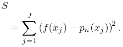
►Here $x_j$, $j=1,2,\mathrm{\dots },J$, is a given set of distinct real points and $J\ge n+1$. … ►In consequence of this structure the number of operations can be reduced to $nm=n{\log }_{2}n$ operations. … ►For many applications a spline function is a more adaptable approximating tool than the Lagrange interpolation polynomial involving a comparable number of parameters; see §3.3(i), where a single polynomial is used for interpolating $f(x)$ on the complete interval $[a,b]$. … ►The slope of the curve at $(x_0,y_0)$ is tangent to the line between $(x_0,y_0)$ and $(x_1,y_1)$; similarly the slope at $(x_3,y_3)$ is tangent to the line between $x_2,y_2$ and $x_3,y_3$. …

14: 28.23 Expansions in Series of Bessel Functions

… ►

28.23.3 $${\mathrm{me}}_{\nu }^{\prime }(0,h^2){\mathrm{M}}_{\nu }^{(j)}(z,h)=\mathrm{i}\tanh z\sum _{n=-\mathrm{\infty }}^{\mathrm{\infty }}{(-1)}^n(\nu +2n)c_{2n}^{\nu }(h^2){𝒞}_{\nu +2n}^{(j)}(2h\cosh z),$$

ⓘ

Symbols:

${\mathrm{me}}_n(z,q)$: Mathieu function, $\cosh z$: hyperbolic cosine function, $\tanh z$: hyperbolic tangent function, $\mathrm{i}$: imaginary unit, ${\mathrm{M}}_{\nu }^{(j)}(z,h)$: modified Mathieu function, $h$: parameter, $n$: integer, $j$: integer, $z$: complex variable, $\nu$: complex parameter, $c_{2m}(q)$: coefficients and ${𝒞}_{\mu }^{(j)}$: cylinder functions

Permalink:

http://dlmf.nist.gov/28.23.E3

Encodings:

pMML, png, TeX

See also:

Annotations for §28.23 and Ch.28

… ►

28.23.10 $${\mathrm{Ms}}_{2m+1}^{(j)}(z,h)={(-1)}^m{\left({\mathrm{se}}_{2m+1}^{\prime }(0,h^2)\right)}^{-1}\tanh z\sum _{\mathrm{\ell }=0}^{\mathrm{\infty }}{(-1)}^{\mathrm{\ell }}(2\mathrm{\ell }+1)B_{2\mathrm{\ell }+1}^{2m+1}(h^2){𝒞}_{2\mathrm{\ell }+1}^{(j)}(2h\cosh z),$$

ⓘ

Symbols:

${\mathrm{se}}_n(z,q)$: Mathieu function, $\cosh z$: hyperbolic cosine function, $\tanh z$: hyperbolic tangent function, ${\mathrm{Ms}}_n^{(j)}(z,h)$: radial Mathieu function, $m$: integer, $h$: parameter, $j$: integer, $z$: complex variable, ${𝒞}_{\mu }^{(j)}$: cylinder functions and $B_m(q)$: Fourier coefficient

Permalink:

http://dlmf.nist.gov/28.23.E10

Encodings:

pMML, png, TeX

See also:

Annotations for §28.23 and Ch.28

… ►

28.23.12 $${\mathrm{Ms}}_{2m+2}^{(j)}(z,h)={(-1)}^m{\left({\mathrm{se}}_{2m+2}^{\prime }(0,h^2)\right)}^{-1}\tanh z\sum _{\mathrm{\ell }=0}^{\mathrm{\infty }}{(-1)}^{\mathrm{\ell }}(2\mathrm{\ell }+2)B_{2\mathrm{\ell }+2}^{2m+2}(h^2){𝒞}_{2\mathrm{\ell }+2}^{(j)}(2h\cosh z),$$

ⓘ

Symbols:

${\mathrm{se}}_n(z,q)$: Mathieu function, $\cosh z$: hyperbolic cosine function, $\tanh z$: hyperbolic tangent function, ${\mathrm{Ms}}_n^{(j)}(z,h)$: radial Mathieu function, $m$: integer, $h$: parameter, $j$: integer, $z$: complex variable, ${𝒞}_{\mu }^{(j)}$: cylinder functions and $B_m(q)$: Fourier coefficient

Permalink:

http://dlmf.nist.gov/28.23.E12

Encodings:

pMML, png, TeX

See also:

Annotations for §28.23 and Ch.28

… ►When $j=2,3,4$ the series in the even-numbered equations converge for $\mathrm{\Re }z>0$ and $|\cosh z|>1$, and the series in the odd-numbered equations converge for $\mathrm{\Re }z>0$ and $|\sinh z|>1$. …

15: 23.20 Mathematical Applications

… ►The addition law states that to find the sum of two points, take the third intersection with $C$ of the chord joining them (or the tangent if they coincide); then its reflection in the $x$-axis gives the required sum. … ►To determine $T$, we make use of the fact that if $(x,y)\in T$ then $y^2$ must be a divisor of $\mathrm{\Delta }$; hence there are only a finite number of possibilities for $y$. … ►

§23.20(v) Modular Functions and Number Theory

►For applications of modular functions to number theory see §27.14(iv) and Apostol (1990). …

16: 25.5 Integral Representations

… ►

25.5.7 $$\zeta \left(s\right)=\frac{1}{2}+\frac{1}{s-1}+\sum _{m=1}^n\frac{B_{2m}}{(2m)!}{\left(s\right)}_{2m-1}+\frac{1}{\mathrm{\Gamma }\left(s\right)}{\int }_0^{\mathrm{\infty }}\left(\frac{1}{{\mathrm{e}}^x-1}-\frac{1}{x}+\frac{1}{2}-\sum _{m=1}^n\frac{B_{2m}}{(2m)!}{x}^{2m-1}\right)\frac{x^{s-1}}{{\mathrm{e}}^x}dx,$$ $\mathrm{\Re }s>-(2n+1)$, $n=1,2,3,\mathrm{\dots }$.

ⓘ

Symbols:

$B_n$: Bernoulli numbers, $O\left(x\right)$: order not exceeding, $\mathrm{\Gamma }\left(z\right)$: gamma function, ${\left(a\right)}_n$: Pochhammer’s symbol (or shifted factorial), $\zeta \left(s\right)$: Riemann zeta function, $dx$: differential of $x$ , $\mathrm{e}$: base of natural logarithm, $!$: factorial (as in $n!$), $\int$: integral, $\mathrm{\Re }$: real part, $m$: nonnegative integer, $n$: nonnegative integer, $x$: real variable and $s$: complex variable

Keywords:

improper integral, integral representation

Proof sketch:

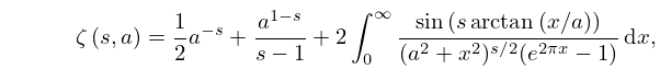
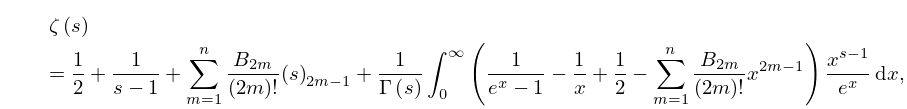
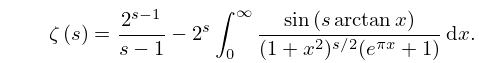
Derivable from (25.5.6) by adding and subtracting ${\sum }_{m=1}^n{B}_{2m}{x}^{2m-1}/(2m)!$ in the integrand, using (5.2.1), (5.2.5), and recognizing that ${({\mathrm{e}}^x-1)}^{-1}-x^{-1}+1/2-{\sum }_{m=1}^n{B}_{2m}{x}^{2m-1}/(2m)!=O\left(x^{2n+1}\right)$ as $x\to 0$, demonstrating the region of convergence.

Referenced by:

Erratum (V1.0.9) for Chapters 7, 25

Permalink:

http://dlmf.nist.gov/25.5.E7

Encodings:

pMML, png, TeX

Notational Change (effective with 1.0.9):

We have rewritten the original summation ${\sum }_{m=1}^n\frac{B_{2m}}{(2m)!}\frac{\mathrm{\Gamma }\left(s+2m-1\right)}{\mathrm{\Gamma }\left(s\right)}$ more concisely as ${\sum }_{m=1}^n\frac{B_{2m}}{(2m)!}{\left(s\right)}_{2m-1}$ using the Pochhammer symbol.

See also:

Annotations for §25.5(i), §25.5 and Ch.25

… ►

25.5.10 $$\zeta \left(s\right)=\frac{2^{s-1}}{1-2^{1-s}}{\int }_0^{\mathrm{\infty }}\frac{\cos \left(s\arctan x\right)}{{(1+x^2)}^{s/2}\cosh \left(\frac{1}{2}\pi x\right)}dx.$$

ⓘ

Symbols:

$\zeta \left(s\right)$: Riemann zeta function, $\pi$: the ratio of the circumference of a circle to its diameter, $\cos z$: cosine function, $dx$: differential of $x$ , $\cosh z$: hyperbolic cosine function, $\int$: integral, $\arctan z$: arctangent function, $x$: real variable and $s$: complex variable

Keywords:

improper integral, integral representation

Sources:

Lindelöf (1905, (6), p. 98); with $x=2t$; Erdélyi et al. (1953a, (1.12.15), p. 33)

Permalink:

http://dlmf.nist.gov/25.5.E10

Encodings:

pMML, png, TeX

See also:

Annotations for §25.5(i), §25.5 and Ch.25

►

25.5.11 $$\zeta \left(s\right)=\frac{1}{2}+\frac{1}{s-1}+2{\int }_0^{\mathrm{\infty }}\frac{\sin \left(s\arctan x\right)}{{(1+x^2)}^{s/2}({\mathrm{e}}^{2\pi x}-1)}dx.$$

ⓘ

Symbols:

$\zeta \left(s\right)$: Riemann zeta function, $\pi$: the ratio of the circumference of a circle to its diameter, $dx$: differential of $x$ , $\mathrm{e}$: base of natural logarithm, $\int$: integral, $\arctan z$: arctangent function, $\sin z$: sine function, $x$: real variable and $s$: complex variable

Keywords:

improper integral, integral representation

Sources:

Lindelöf (1905, (3), p. 97); Erdélyi et al. (1953a, (1.12.12), p. 33)

Permalink:

http://dlmf.nist.gov/25.5.E11

Encodings:

pMML, png, TeX

See also:

Annotations for §25.5(i), §25.5 and Ch.25

►

25.5.12 $$\zeta \left(s\right)=\frac{2^{s-1}}{s-1}-2^s{\int }_0^{\mathrm{\infty }}\frac{\sin \left(s\arctan x\right)}{{(1+x^2)}^{s/2}({\mathrm{e}}^{\pi x}+1)}dx.$$

ⓘ

Symbols:

$\zeta \left(s\right)$: Riemann zeta function, $\pi$: the ratio of the circumference of a circle to its diameter, $dx$: differential of $x$ , $\mathrm{e}$: base of natural logarithm, $\int$: integral, $\arctan z$: arctangent function, $\sin z$: sine function, $x$: real variable and $s$: complex variable

Keywords:

improper integral, integral representation

Source:

Lindelöf (1905, (4), p. 98); with $x=2t$

Permalink:

http://dlmf.nist.gov/25.5.E12

Encodings:

pMML, png, TeX

See also:

Annotations for §25.5(i), §25.5 and Ch.25

…

17: Errata

… ►This release increments the minor version number and contains considerable additions of new material and clarifications. … ►This release increments the minor version number and contains considerable additions of new material and clarifications. These additions were facilitated by an extension of the scheme for reference numbers; with “_” introducing intermediate numbers. These enable insertions of new numbered objects between existing ones without affecting their permanent identifiers and URLs. … ►

These equations have been rewritten to improve the numerical computation of $\arctan x$.

…

18: 31.2 Differential Equations

… ►The total number of free parameters is six. … ►

31.2.6 $$\frac{d^{2}w}{{d\theta }^2}+\left((2\gamma -1)\cot \theta -(2\delta -1)\tan \theta -\frac{ϵ\sin \left(2\theta \right)}{a-{\sin }^2\theta }\right)\frac{dw}{d\theta }+4\frac{\alpha \beta {\sin }^2\theta -q}{a-{\sin }^2\theta }w=0.$$

ⓘ

Symbols:

$\cot z$: cotangent function, $\frac{df}{dx}$: derivative of $f$ with respect to $x$ , $\sin z$: sine function, $\tan z$: tangent function, $\gamma$: real or complex parameter, $\delta$: real or complex parameter, $ϵ$: real or complex parameter, $a$: complex parameter, $q$: real or complex parameter, $\alpha$: real or complex parameter and $\beta$: real or complex parameter

Permalink:

http://dlmf.nist.gov/31.2.E6

Encodings:

pMML, png, TeX

See also:

Annotations for §31.2(iii), §31.2 and Ch.31

… ►

31.2.11 $$d^{2}W/{d\xi }^2+\left(H+b_0\mathrm{\wp }\left(\xi \right)+b_1\mathrm{\wp }\left(\xi +{\omega }_1\right)+b_2\mathrm{\wp }\left(\xi +{\omega }_2\right)+b_3\mathrm{\wp }\left(\xi +{\omega }_3\right)\right)W=0,$$

ⓘ

Defines:

$W(\xi )$: solution (locally)

Symbols:

$\mathrm{\wp }\left(z\right)$ (= $\mathrm{\wp }\left(z|𝕃\right)$ = $\mathrm{\wp }(z;g_2,g_3)$): Weierstrass $\mathrm{\wp }$-function, $\frac{df}{dx}$: derivative of $f$ with respect to $x$ , ${\omega }_j$: nonzero complex number, $𝕃$: lattice, $b_j$: coefficients and $H$

Permalink:

http://dlmf.nist.gov/31.2.E11

Encodings:

pMML, png, TeX

See also:

Annotations for §31.2(iv), §31.2(iv), §31.2 and Ch.31

…

19: 18.21 Hahn Class: Interrelations

… ►

18.21.10 $$\underset{t\to \mathrm{\infty }}{lim}{t}^{-n}{p}_n(x-t;\lambda +it,-t\tan \varphi ,\lambda -it,-t\tan \varphi )=\frac{{(-1)}^n}{{(\cos \varphi )}^n}{P}_n^{(\lambda )}(x;\varphi ).$$

ⓘ

Symbols:

$P_n^{(\lambda )}(x;\varphi )$: Meixner–Pollaczek polynomial, $p_n(x;a,b,\overline{a},\overline{b})$: continuous Hahn polynomial, $\cos z$: cosine function, $\tan z$: tangent function, $t$: real variable, $n$: nonnegative integer and $x$: real variable

Referenced by:

§18.21(ii), §18.22(ii), §18.22(iii)

Permalink:

http://dlmf.nist.gov/18.21.E10

Encodings:

pMML, png, TeX

See also:

Annotations for §18.21(ii), §18.21(ii), §18.21 and Ch.18

… ►

►►

Figure 18.21.1: Askey scheme. The number of free real parameters is zero for Hermite polynomials. … Magnify

20: Bibliography R

… ►

Topics in Analytic Number Theory. Springer-Verlag, New York.

ⓘ

Notes:

Edited by E. Grosswald, J. Lehner and M. Newman, Die Grundlehren der mathematischen Wissenschaften, Band 169

External Links:

MathReview (H. Halberstam), ZentralBlatt

Referenced by:

§1.8(iv), §20.7(viii), §20.7(viii), Ch.24.

Encodings:

BibTeX

… ►

Some properties of Bernoulli’s numbers (J. Indian Math. Soc. 3 (1911), 219–234.). In Collected Papers,

ⓘ

Referenced by:

§24.7(i).

Encodings:

BibTeX

… ►

Roots of $\tan x=x$ .

ⓘ

Notes:

10 typewritten pages deposited in the UMT file at Lawrence Berkeley Laboratory, University of California, Berkeley, CA.

Referenced by:

§4.46.

Encodings:

BibTeX

… ►

Elementary Number Theory and its Applications. 5th edition, Addison-Wesley, Reading, MA.

ⓘ

External Links:

ISBN 0-201-87073-8, MathReview (Norman J. Richert)

Referenced by:

§27.17.

Encodings:

BibTeX

…